iris.scaled <- scale(iris[, -5])Workshop 2: Clustering
Clustering is one of the main tools in unsupervised learning. It provides a powerful and versatile technique for discovering hidden patterns and inherent structures within data sets. Clustering algorithms group similar data points together based on inherent similarities or distances, revealing natural subdivisions within the data set. By facilitating the automatic exploration of data relationships, clustering contributes to a deeper understanding of complex datasets and supports informed decision-making processes in various real-world applications.
There are many clustering algorithms. We will begin by exploring the most popular ones, starting with K-means and K-medoids (a robust alternative to K-means). We will examine the algorithm behind K-means and learn how to combine PCA with K-means clustering for more effective visualization. By the end of the workshop, we will also understand why K-medoids is robust to outliers. If time permits, we will explore model-based clustering, specifically the Gaussian mixture model.
K-means
Here we use Iris dataset to apply the K-means clustering. Recall that iris data set has a natural category for the species (three levels: Setosa, Versicolor, Virginica), which is helpful for clustering. A natural motivating question for our exploration is:
We first scale the data.
Task: Does scaling make sense to you? Why?
We will use the kmeans() command, which is already implemented in R. Let’s explore its features:
?kmeansWe can see that the command requires us to specify the “centers”, or at least the number of clusters.
We use a screeplot measuring the effectiveness of the clusters weighted by the number of clusters.
In practice, this is accomplished using the fviz_nbclust() function from the factoextra package.
library(factoextra)fviz_nbclust(iris.scaled, kmeans, method = "wss") 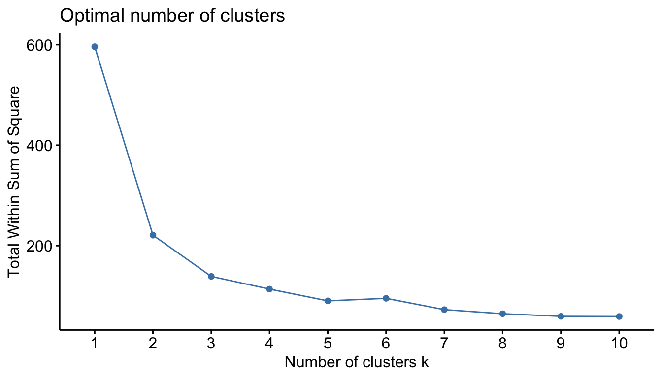
This Figure is treated the same way as we did with the scree plot. We locate the bend (elbow) in the plot. This seems to be at \(k=3\). So we will use three clusters for the analysis.
The model can be fitted as follows:
# Compute k-means with k = 3
set.seed(123)
km.res <- kmeans(iris.scaled, 3, nstart = 25)
The option nstart = 25 means that R will try 25 different random initial cluster assignments and then select the best results corresponding to the one with the lowest within cluster variation (more of this in lectures).
names(km.res)[1] "cluster" "centers" "totss" "withinss" "tot.withinss"
[6] "betweenss" "size" "iter" "ifault" The output of clustering consists of 9 categories. The most important are:
- “cluster”: the assignment of a number from 1 to 3 (the cluster) to each observation
- “centers”: the cluster means for each cluster. The algorithm minimizes the distances from these centers
- “withinss” : the sum of square distances of points from centers of a cluster for each cluster
One measure of effectiveness is the variability accounted for with this clustering method.
Task
Extract appropriate quantity from the object km.res to compute the percentage variability explained by the clusters. Interpret the results.
Solution
We can use the table() function in R to compare the true class labels to the class labels obtained by clustering.
table(iris$Species, km.res$cluster)
              1  2  3
  setosa     50  0  0
  versicolor  0 39 11
  virginica   0 14 36
All 50 Setosa observations are correctly assigned by this clustering. Out of the 50 observations from Versicolor, 39 agree with the label while 11 observations are labeled as Virginica. 36 observations from Virginica are put in the correct cluster. Overall, 83.3% correct classification is obtained from the algorithm (((50+39+36)/150)*100).
If the number of variables is greater than 2, then visualization is a bit of a challenge. However, when two principal components explain a good portion of the variability, we can use PCA to gain an effective visualization. This is what fviz_cluster() does in practice:
# Visualise kmeans clustering
fviz_cluster(km.res, iris[, -5], ellipse.type = "norm")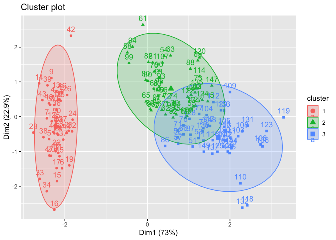
This visualization is not perfect, and we should always remember that clustering is computed in the original feature space, not in the plane spanned by PC1 and PC2.
K-medoids
K-medoids algorithm is a clustering approach related to K-means clustering for partitioning a data set into \(k\) clusters. In K-medoids clustering, each center is represented by one of the data point in the cluster. These points are named cluster medoids. Medoid corresponds to the most centrally located point in the cluster. While K-means takes the average (centroid) of the \(k^\text{th}\) cluster to minimise the total within cluster variation, K-medoids replaces this by an optimisation step which restricts the search space to the observations within the \(k^\text{th}\) cluster (see lectures for precise details).
Task
The main advantage of K-medoids over K-means clustering is that it is less sensitive to noise and outliers. Can you think of why?
Solution
The most common K-medoids clustering methods is the PAM algorithm (Partitioning Around Medoids). We will use a faster implementation of PAM using the CLARA (Clustering Large Applications) function within the cluster package in this workshop. Other packages for K-medoids in R are kmedoids() function in clue package (Cluster Ensembles) and pamk() in the fpc package.
The model is fitted as:
clara(x, k, metric="euclidean" stand=FALSE)
where:
x: data matrix or dissimilarity matrix
k: number of clusters
metric:
euclideanormanhattandistancestand: if set to TRUE, the variables are scaled to have unit variance before the analysis takes place.
library(cluster)
iris.scaled <- scale(iris[, -5])
pam.res <- clara(iris.scaled, k=3)

names(pam.res)
[1] "sample" "medoids" "i.med" "clustering" "objective"
[6] "clusinfo" "diss" "call" "silinfo" "data" We are especially interested in medoids which shows the objects representing cluster and clustering which gives a vector containing the cluster number of each object.
pam.res$medoids Sepal.Length Sepal.Width Petal.Length Petal.Width
[1,] -0.89767388 0.7861738 -1.27910398 -1.3110521482
[2,] -0.05233076 -0.8198233 0.08043967 0.0008746178
[3,] 0.79301235 -0.1315388 0.81685914 1.0504160307pam.res$i.med[1] 40 83 148Observe that the flowers n. 40, 83 and 148 from the scaled iris data correspond to the medoids shown above. You can easily check this as iris.scaled[c(40,83,148),]
The cluster for the observations can be obtained as:
pam.res$clustering [1] 1 1 1 1 1 1 1 1 1 1 1 1 1 1 1 1 1 1 1 1 1 1 1 1 1 1 1 1 1 1 1 1 1 1 1 1 1
[38] 1 1 1 1 2 1 1 1 1 1 1 1 1 3 3 3 2 3 2 3 2 3 2 2 2 2 2 2 3 2 2 2 2 3 2 2 2
[75] 2 3 3 3 2 2 2 2 2 2 2 3 3 2 2 2 2 2 2 2 2 2 2 2 2 2 3 3 3 3 3 3 2 3 3 3 3
[112] 3 3 2 3 3 3 3 3 2 3 3 3 3 3 3 3 3 3 3 3 3 3 3 2 3 3 3 3 3 3 3 3 3 3 3 3 3
[149] 3 3We use the table() function to compare the true class labels and the class labels obtained by K-medoids clustering. Does this result offer any improvement over the K-means results obtained above?
table(iris$Species, pam.res$clustering)
              1  2  3
  setosa     49  1  0
  versicolor  0 37 13
  virginica   0  4 46
An alternative option to get the same result:
We notice that our clustering misclassifies 1 of the setosa species as versicolor (49 out of 50 correctly classified). Virginica species got some improvement over the previous K-means results, only 4 observations are misclassified whereas 14 observations are misclassified in K-means. Overall, 88% ((49+37+46)/150*100) correct classification is obtained under K-medoids whereas 83.3% correct classification was obtained for K-means.
We can use the fviz_cluster function to visualise the clusters as before.
library(factoextra)
fviz_cluster(pam.res, iris[, -5], ellipse.type = "norm")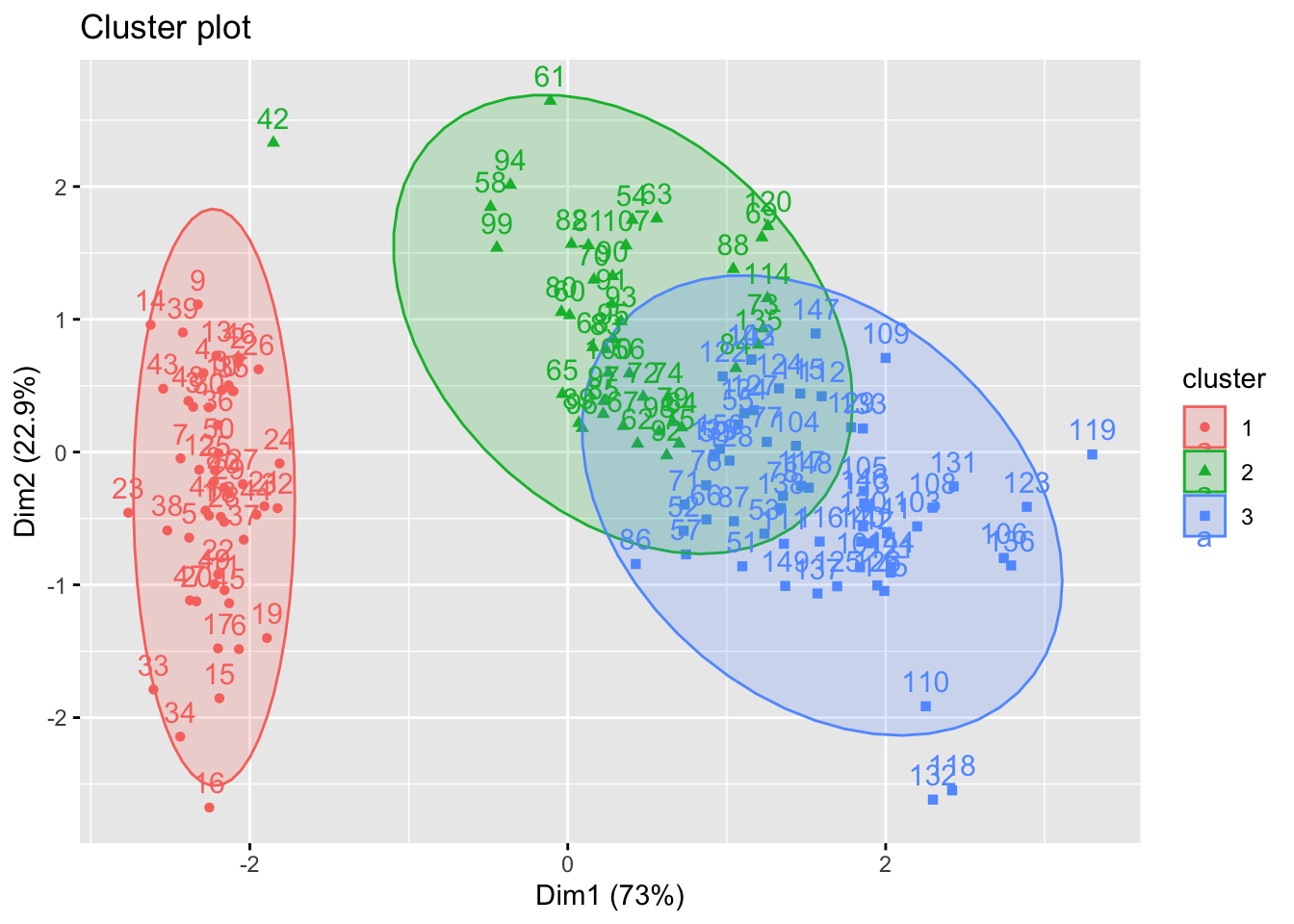
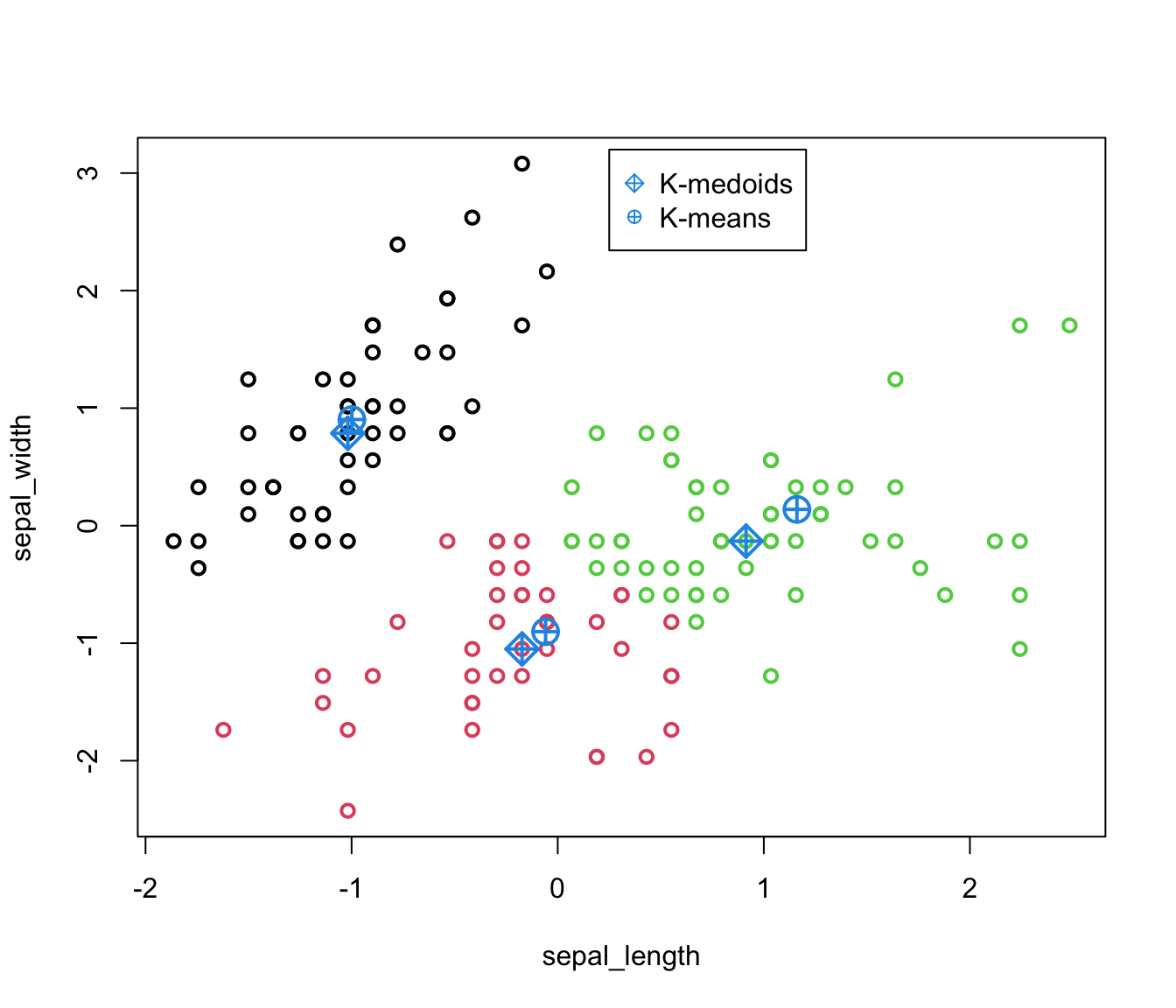
We show in the figure below that the medoids are indeed a data point whereas centroids are not.
Silhouette measure
We were introduced to the Silhouette measure in Practical 1. It is a method commonly used to determine the optimal number of clusters. Let us now revisit the solutions to the practicals and review a few lecture slides on the theory behind it, using the Iris dataset.
We will then demonstrate how to visualise this method for the Iris dataset using the following three algorithms: K-means, K-medoids, and Hierarchical clustering (with appropriate linkage).
Silhouette width is a quantity associated with every observation inside a cluster. For each algorithm, we can compute the overall average silhouette width inside each cluster. The maximum of these values gives the optimal number of cluster (for each algorithm).
#K-means
fviz_nbclust(iris.scaled, kmeans, method = "silhouette")+
  labs(title = "K-means")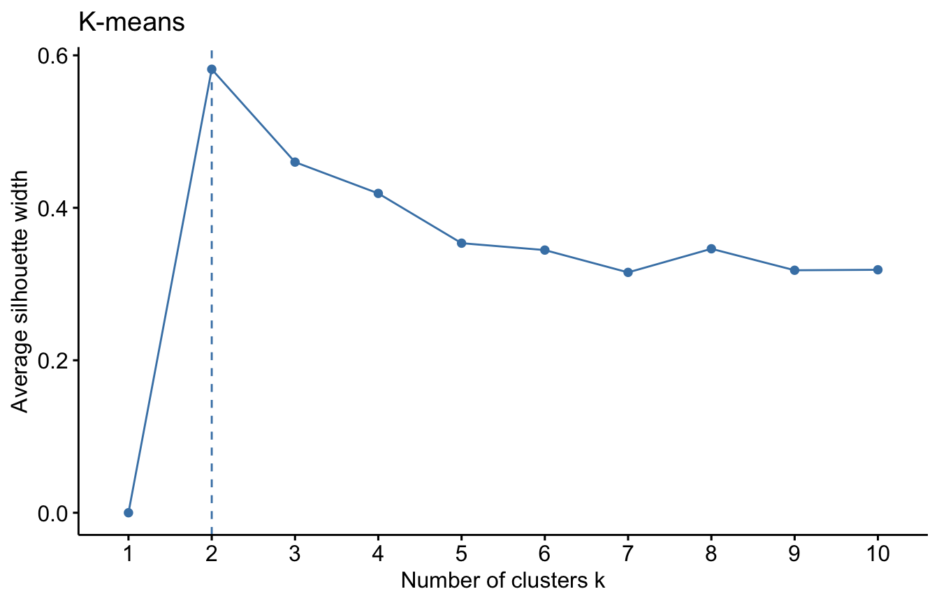
#K-medoids
fviz_nbclust(iris.scaled, clara, method = "silhouette")+
  labs(title = "K-medoids")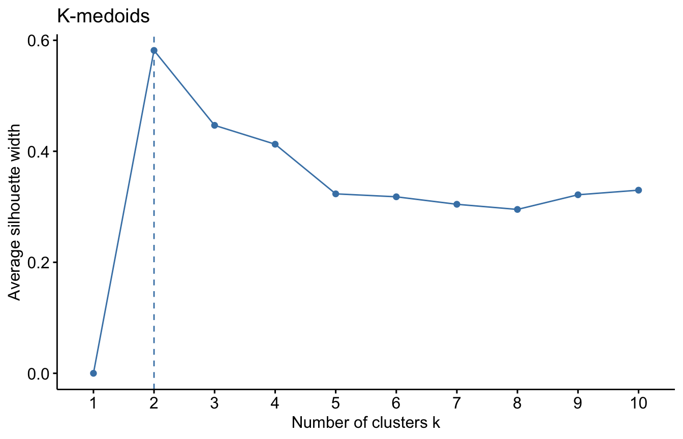
# Hierarchical
fviz_nbclust(iris.scaled, hcut, method = "silhouette")+
  labs(title = "Hierarchical")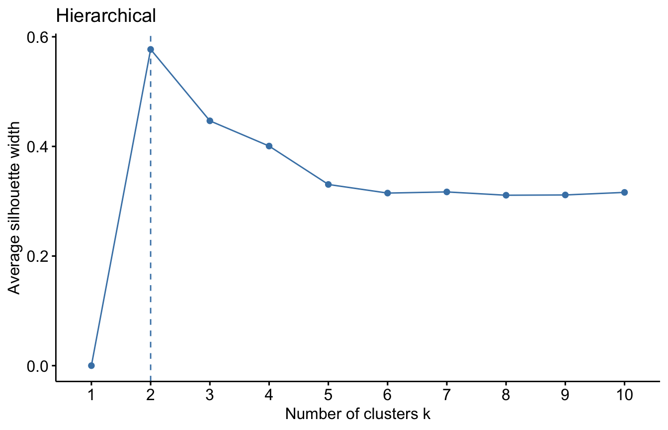
The optimal number of clusters is two!
It is not so surprising, given that the observations from the Versicolor and Virginica varieties cluster well together. The real reason we chose 3 clusters in the analysis of the Iris data set is that we knew there were three different varieties. So, prior knowledge is an important factor in choosing the number of clusters as much as quantitative measures such as Silhouette.
We used the Silhouette measure to select optimal number of clusters within a method. We can select the optimal number of clusters as well as the optimal algorithm using a general validation method implemented in the clValid package. For more info about this, see HERE.
Model-based clustering: the Gaussian mixture model (optional)
The clustering methods that we have discussed so far neither involve any sort of model nor are based on a density estimate. Model-based clustering considers the data as coming from a distribution that is a mixture of two or more clusters. In the Gaussian mixture model, each cluster \(C_k\) is modelled by a random variable with a multivariate normal distribution \(N_p(\mu_{k}, \Sigma_{k})\). Recall that we have:
- \(\mu_{k}:\) mean vector for the \(k\)-th cluster
- \(\Sigma_{k}:\) covariance matrix for the \(k\)-th cluster
Aside
To get a better idea of how such a distribution looks like, we can visualize the joint probability distribution in some simple cases, such as the one of 3 clusters and 2 variables.
# Part (a) generate data:
#
K = 3  # the number of classes
n = 20 # the number of samples per class
p = 2 # the number of variables

set.seed(123)
# Create data for class 1:
X_1 = matrix( rnorm(n*p), nrow=n, ncol=p )
for( row in 1:n ){
  X_1[row,] = X_1[row,] + rep( 2, p )
}

# Create data for class 2:
X_2 = matrix( rnorm(n*p), nrow=n, ncol=p )
for( row in 1:n ){
  X_2[row,] = X_2[row,] + rep( -2, p )
}

# Create data for class 3:
X_3 = matrix( rnorm(n*p), nrow=n, ncol=p )
for( row in 1:n ){
  X_3[row,] = X_3[row,] + c( rep( 1, p/2 ), rep( -1, p/2 ) )
}

X <- rbind(X_1, X_2, X_3)library(mclust)
ex.mc <- Mclust(X, G=3)
plot(ex.mc, what = "density")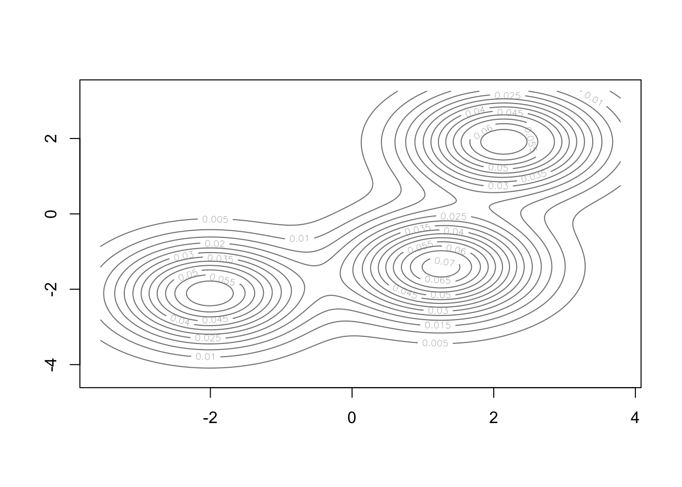
The model parameters \(\mu_{k}\) and \(\Sigma_{k}\) can be estimated using the Expectation-Maximisation (EM) algorithm. As a result, each observation point \(x\) comes with a probability of belonging to a cluster \(p_k(x)\). These probabilities satisfy
\[p_1(x)+\dots+p_n(x)=1,\] where \(n\) is the total number of clusters, as we are assuming that all points belong to some cluster. This method has been implemented in the mclust package in R.
Since the model is based on maximum likelihood estimation, criteria such as BIC (Bayesian Information Criterion) and AIC (Akaike Information Criterion) can be used for the selection of the number of clusters.
We briefly recall the form of these two criteria:
\[AIC = -2logL +2p\] \[BIC = -2logL +log(n)p\] where \(logL\) is the model log-likelihood, \(p\) is the number of parameters and \(n\) is the number of observations. In general, we want these quantities to be small. The model with the smallest value of the criterion is selected as the best.
BIC is often used for selecting the number of clusters.
Let us see how good model based clustering is on the iris data set.
iris.scaled <- scale(iris[, -5]) # Standardise the data
mc <- Mclust(iris.scaled, G = 3) # Model-based-clustering, G=3 indicates a request for 3 clusters
summary(mc)
----------------------------------------------------
Gaussian finite mixture model fitted by EM algorithm
----------------------------------------------------
Mclust VVV (ellipsoidal, varying volume, shape, and orientation) model with 3
components:
log-likelihood n df BIC ICL
-288.5255 150 44 -797.519 -800.7391
Clustering table:
1 2 3
50 45 55 The result indicates that there are 50 observations in cluster 1, 45 in cluster 2 and 55 in cluster 3.
We can examine the variables created within object mc:
names(mc) [1] "call" "data" "modelName" "n"
[5] "d" "G" "BIC" "loglik"
[9] "df" "bic" "icl" "hypvol"
[13] "parameters" "z" "classification" "uncertainty" The value that is of utmost importance in the object created is classification. These are the newly created clusters.
mc$classification [1] 1 1 1 1 1 1 1 1 1 1 1 1 1 1 1 1 1 1 1 1 1 1 1 1 1 1 1 1 1 1 1 1 1 1 1 1 1
[38] 1 1 1 1 1 1 1 1 1 1 1 1 1 2 2 2 2 2 2 2 2 2 2 2 2 2 2 2 2 2 2 3 2 3 2 3 2
[75] 2 2 2 3 2 2 2 2 2 3 2 2 2 2 2 2 2 2 2 2 2 2 2 2 2 2 3 3 3 3 3 3 3 3 3 3 3
[112] 3 3 3 3 3 3 3 3 3 3 3 3 3 3 3 3 3 3 3 3 3 3 3 3 3 3 3 3 3 3 3 3 3 3 3 3 3
[149] 3 3
As a small task, use the table() function in R to compare the true class labels to the class labels obtained from mclust. Does this result offer any improvement over the K-means clustering results?
              1  2  3
  setosa     50  0  0
  versicolor  0 45  5
  virginica   0  0 50
If you implemented this correctly, then Setosa is correctly classified (50 out of 50 correctly classified). 5 observations are misclassified in Versicolor (45 out of 50 correctly classified). Overall, 97% correct classification is obtained under the model-based clustering, whereas it was 88% under K-medoids and 83.3% under K-means.
You can obtain four different types of plot from the mc object that was created.
Model-based clustering plots:
1: BIC
2: classification
3: uncertainty
4: density
We can plot the classification as follows:
plot(mc, what = "classification")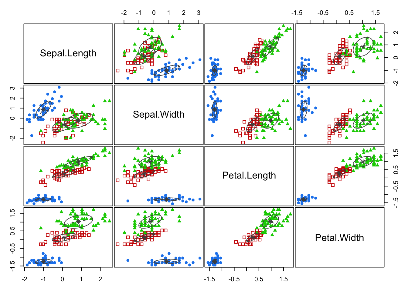
Let us compare the former plot with the one given by selecting the “uncertainty” option:
plot(mc, what = "uncertainty")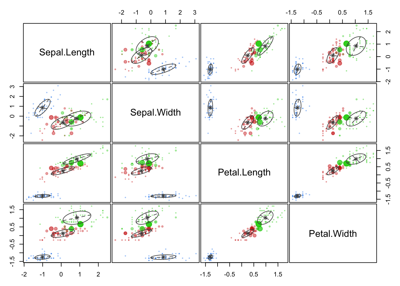
In the second one, the classification uncertainty of a point is highlighted by the dimension of the corresponding dot.
We can identify the 5 observations that were misclassified and calculate the classification error rate as follows.
classError(mc$classification, iris[,5])$misclassified
[1] 69 71 73 78 84
$errorRate
[1] 0.03333333
Then, we can have a look at the plot of density functions:
plot(mc, what = "density")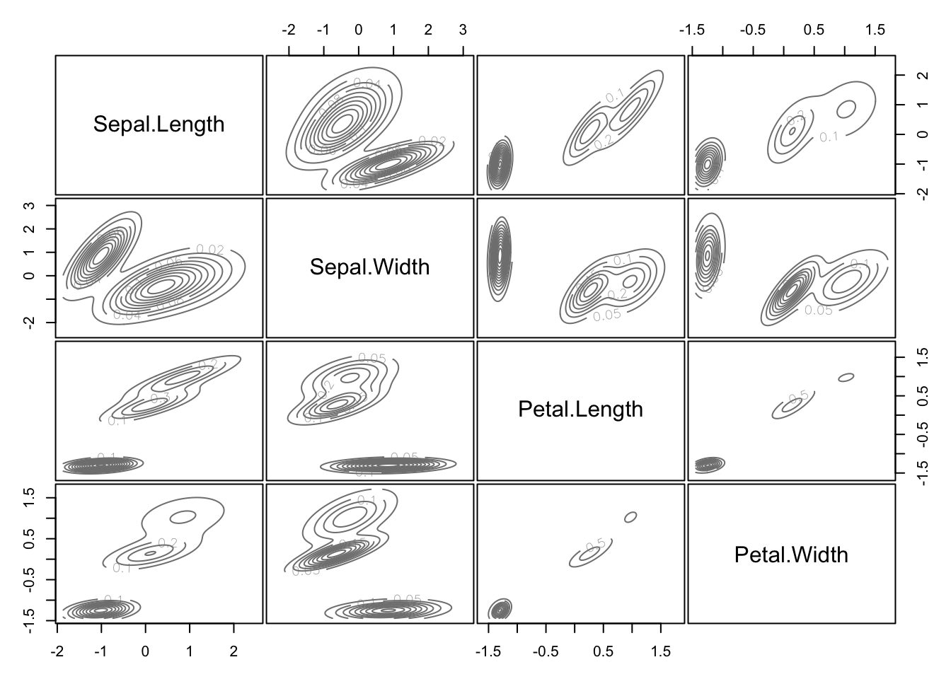
These are the probability density functions of the multivariate normals appearing in the model.
Finally, here is the BIC plot:
plot(mc, what = "BIC")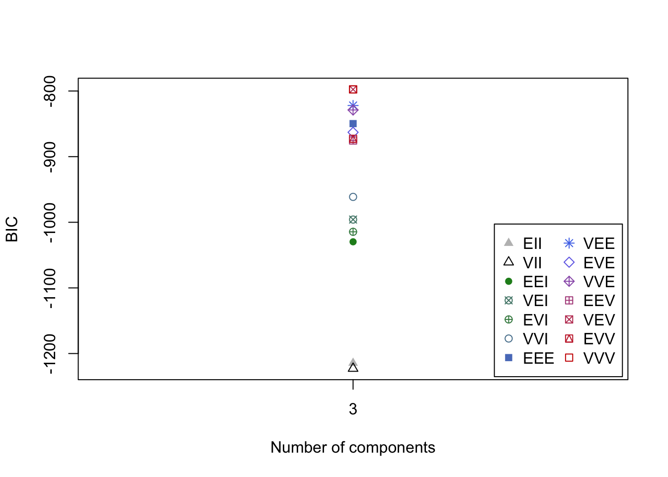
The available model options in mclust package, are represented by identifiers including: EII, VII, EEI, VEI, EVI, VVI, EEE, EEV, VEV and VVV. So, VVV has been used for our example as the option with the best BIC, but the plot shows that there are different options that return a similar value.
What do these letters mean? The first identifier refers to volume, the second to shape and the third to orientation. E stands for “equal”, V for “variable” and I for “coordinate axes”. VEI, for example, implies that the clusters have variable volume, the same shape and orientation equal to coordinate axes. EEE means that the clusters have the same volume, shape and orientation in p-dimensional space. More on this in the Lab!
To enforce VEV as a model option, for example, you can do the following:
mc_option <- Mclust(iris.scaled, G = 3, modelNames = "VEV")Now, let us try to compare the performance of model options VEV, EVE and VEI to VVV.
You are required to fit the models using the three model options, create a classification table and compare the percentage of correct classification with what we obtained for VVV.
mc_option_VEV <- Mclust(iris.scaled, G = 3, modelNames = "VEV")
table(iris[,5], mc_option_VEV$classification)
              1  2  3
  setosa     50  0  0
  versicolor  0  0 50
virginica 0 34 16(50+50+34)/150[1] 0.8933333mc_option_EVE <- Mclust(iris.scaled, G = 3, modelNames = "EVE")
table(iris[,5], mc_option_EVE$classification)
              1  2  3
  setosa     50  0  0
  versicolor  0 50  0
virginica 0 16 34(50+50+34)/150[1] 0.8933333mc_option_VEI <- Mclust(iris.scaled, G = 3, modelNames = "VEI")
table(iris[,5], mc_option_VEI$classification)
              1  2  3
  setosa     50  0  0
  versicolor  0 48  2
virginica 0 4 46(50+48+46)/150[1] 0.96mc_option_VVV <- Mclust(iris.scaled, G = 3, modelNames = "VVV")
table(iris[,5], mc_option_VVV$classification)
              1  2  3
  setosa     50  0  0
  versicolor  0 45  5
virginica 0 0 50(50+45+50)/150[1] 0.9666667The automatically selected model option, VVV is the best with 97% classification accuracy. This is followed by VEI at 96% accuracy. The worst are the first two at 89.3%, although they are still better than all the previous clustering methods (K-means, K-medoids and Hierarchical). Unsurprisingly, model based clustering performs much better when natural clusters are present in the data!
One should use the BIC criterion (higher values are desirable) to select the number of clusters (G). Consider the case below:
mc_bic <- Mclust(iris.scaled, G = 3)
mc_bic$BIC
Bayesian Information Criterion (BIC):
EII VII EEI VEI EVI VVI EEE
3 -1214.525 -1222.844 -1029.733 -995.8343 -1014.515 -961.3205 -849.6448
VEE EVE VVE EEV VEV EVV VVV
3 -822.076 -862.9077 -828.8731 -875.3724 -797.5483 -872.7515 -797.519
Top 3 models based on the BIC criterion:
VVV,3 VEV,3 VEE,3
-797.5190 -797.5483 -822.0760 You will observe that the results included the top 3 model options based on the BIC criterion. In fact, if no number of clusters is specified, the algorithm naturally selects the best options using BIC. The downside of this method is that it takes much longer to run:
mc_bic <- Mclust(iris.scaled)
mc_bic$BIC
Bayesian Information Criterion (BIC):
EII VII EEI VEI EVI VVI EEE
1 -1723.766 -1723.766 -1738.7979 -1738.7979 -1738.7979 -1738.7979 -1046.6559
2 -1344.053 -1325.273 -1259.6457 -1172.9600 -1223.9860 -1074.2293 -904.7750
3 -1214.525 -1222.844 -1029.7330 -995.8343 -1014.5146 -961.3205 -849.6448
4 -1177.163 -1139.392 -1044.1118 -965.1348 -1054.2229 -967.7021 -862.7323
5 -1135.642 -1107.791 -958.6219 -905.0241 -983.5054 -928.1301 -821.5159
6 -1131.245 -1102.864 -910.4787 -892.8517 -990.7497 -923.9756 -826.5558
7 -1119.876 -1053.274 -929.8709 -897.4180 -1030.2038 -983.3316 -849.1854
8 -1124.299 -1059.090 -908.1008 -896.1450 -957.1355 -980.8747 -855.9594
9 -1114.899 -1060.444 -912.9422 -918.7055 -984.5159 -972.5093 -869.7734
VEE EVE VVE EEV VEV EVV VVV
1 -1046.6559 -1046.6559 -1046.6559 -1046.6559 -1046.6559 -1046.6559 -1046.6559
2 -873.0048 -906.9282 -880.7933 -873.6590 -802.5253 -875.0084 -790.6956
3 -822.0760 -862.9077 -828.8731 -875.3724 -797.5483 -872.7515 -797.5190
4 -821.5149 -902.9964 -881.1270 -930.1693 -821.4057 -941.9898 -847.2777
5 NA -901.9539 -853.4148 -877.2201 -837.6111 NA -893.2973
6 -826.2392 -873.0654 -865.1217 -905.4942 -879.2801 NA -971.4786
7 NA -913.1458 -898.7411 -953.7660 -920.8553 -1026.5234 -1023.6106
8 -871.9319 -934.3770 -908.8799 -955.7741 -939.3449 -1048.4311 -1047.3167
9 NA -955.8249 -947.9984 -990.5646 -987.1010 -1099.1226 -1100.3729
Top 3 models based on the BIC criterion:
VVV,2 VVV,3 VEV,3
-790.6956 -797.5190 -797.5483 In summary: model-based clustering allows for mixing between clusters, it is useful to give precise metrics of mis-clustering (hence easier to manage outliers), and more flexibility as we are assigning a probability rather than a certainty.