Factor analysis (FA) is a dimension reduction technique that presents some similarities with PCA, but also marked differences. The most important distinction is that FA not only reduces the dimension, but is also a tool for latent variable modelling: FA explicitly specifies a model relating the observed variables to a smaller set of underlying unobservable factors while PCA is a data transformation tool. As a result, Factor Analysis is more powerful, but also more challenging.
Here we explore how to perform FA using R, how to read and visualize the output, as well as good practices and pitfalls to avoid. For a more theoretical viewpoint on FA, you are referred to the lecture notes.
In R, FA can be performed using either fa() or factanal().
Quality of life data
We will start by testing the factanal() function on the quality of life data provided by WHO. You can download the data set lifexpect.csv from Learn Ultra.
We begin by reading the data into R and analyze its structure.
The data contains measurement for multiple countries and multiple years of variables that are indicators of basic quality of life. We would like to understand, through FA, if unobservable features can be extracted from this setting. The factanal() command requires a specification of the number of factors. For the moment, to keep it simple, we choose 2 factors and select only the last 5 variables.
Call:
factanal(x = dat[, -(1:8)], factors = 2)

Uniquenesses:
Hepatitis.B       Polio  Diphtheria         GDP   Schooling
      0.527       0.494       0.251       0.702       0.405

Loadings:
            Factor1 Factor2
Hepatitis.B 0.684
Polio       0.667   0.248
Diphtheria  0.847   0.177
GDP                 0.541
Schooling   0.230   0.736

               Factor1 Factor2
SS loadings      1.689   0.932
Proportion Var   0.338   0.186
Cumulative Var   0.338   0.524

Test of the hypothesis that 2 factors are sufficient.
The chi square statistic is 1.22 on 1 degree of freedom.
The p-value is 0.27
What do we observe?
Recall from lectures, that FA decomposes the estimated covariance matrix as [ X = LL^+ {} ]
Uniquenesses
The uniquenesses range from 0 to 1. These are the diagonal entries of the matrix \(\Sigma_{\epsilon}\). They are the proportion of variability unexplained by the common factors.
life.fa$uniquenesses
Hepatitis.B       Polio  Diphtheria         GDP   Schooling
  0.5269175   0.4935167   0.2513118   0.7021875   0.4047552
Uniqueness is higher for GDP: the variance of this variable will then remain largely unaccounted for in the factor model.
Uniqueness is low for Diphteria immunisation rates. This means that its variance is mostly accounted for by the factors.
Loadings
The loadings range from -1 to 1. They are the vectors that make up the matrix \(L\) in the model. They show the contributions of each original variable to each of the two factors.
life.fa$loadings
Loadings:
            Factor1 Factor2
Hepatitis.B 0.684
Polio       0.667   0.248
Diphtheria  0.847   0.177
GDP                 0.541
Schooling   0.230   0.736

               Factor1 Factor2
SS loadings      1.689   0.932
Proportion Var   0.338   0.186
Cumulative Var   0.338   0.524
We see that the first factor aims to explain the rate of immunisation more than the socioeconomic factors. We could say that this measures “immunisation policy”. The second factor is somehow complementary to that, and we could say that this measures “country development”. Some entries are left blank: these are those that are too small to contribute to the factor.
The sum of the squares of the loadings gives the proportion of variance of each variable explained by the factor model. This is also called the communality.
apply(life.fa$loadings^2, 1, sum)
Hepatitis.B       Polio  Diphtheria         GDP   Schooling
  0.4730830   0.5064836   0.7486882   0.2978126   0.5952448
Note that, by our model formula, this can also be obtained by subtracting the uniquenesses from the vector whose entries are all equal to 1.
1- life.fa$uniquenesses
Hepatitis.B       Polio  Diphtheria         GDP   Schooling
  0.4730825   0.5064833   0.7486882   0.2978125   0.5952448
Variance explained
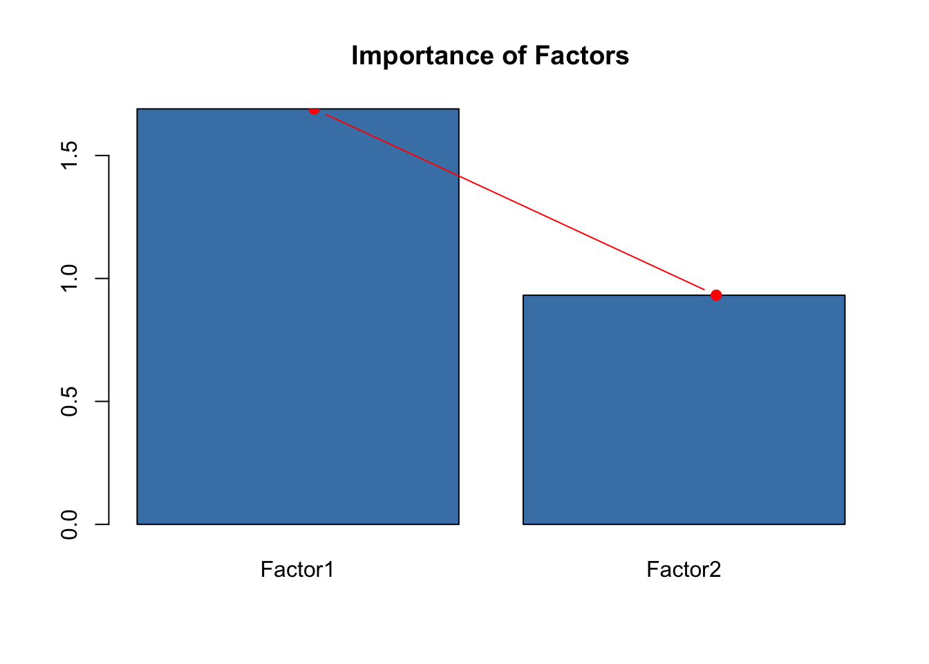
In the “loadings” part of the output, we observe a table showing the variance explained. The row Cumulative Var gives the cumulative proportion of variance explained, while the row Proportion Var gives the proportion of variance explained by each factor. The row SS loadings gives the sum of the squared loadings, which is an indication of the importance of a particular factor. We can visualize this with a screeplot.
L <- life.fa$loadingsSS <-apply(L^2, 2, sum)barplot(SS, col='steelblue' , main="Importance of Factors")lines(x =c(.75,2), SS, type="b", pch=19, col ="red")
We do not worry too much that the cumulative proportion of variance explained is lower than 80% here: we are trying to analyze underlying factors rather than finding subspaces maximizing the variance, so this is to be expected.
Likelihood ratio test
The final part of the factanal() output shows the performance of the model in the likelihood ratio test, which is relevant because the factors are computed using a maximum likelihood estimate. Likelihood ratio test is a hypothesis test with respect to the following null hypothesis:
\(H_0\): 2 factors are enough to capture the information contained in the data set.
In standard hypothesis testing, we reject \(H_0\) when the p value is small enough (<0.05), and we do not reject it otherwise. If we reject \(H_0\), we might need to account for more factors; if we fail to reject \(H_0\) (as in our case above) then it is very likely that there are enough factors for the model to be appropriate. In both cases the analysis might be appropriate, but in the first case we should observe that we are analyzing only some of the possible factors.
Visualization
To visualize our data in the space of factors, we need to determine the scores.
Uniquenesses show that a good portion of variance is accounted by the model for under 5 deaths, Diphtheria immunization and Schooling, while the model fails to account for most of the variance of Adult mortality and GDP. This does not mean that these variables don’t play a role, though, as the factor model aims at explaining covariances too.
Loadings show that the first factor is a combination mostly of immunization rates, the second factor has a mixed contribution accounting positively for socioeconomical factors and negatively for mortality factors (so, “wealth with effective death prevention” could be a label for this factor) and the third factor predominantly represents under 5 deaths (possible label: “adjusted infant mortality”).
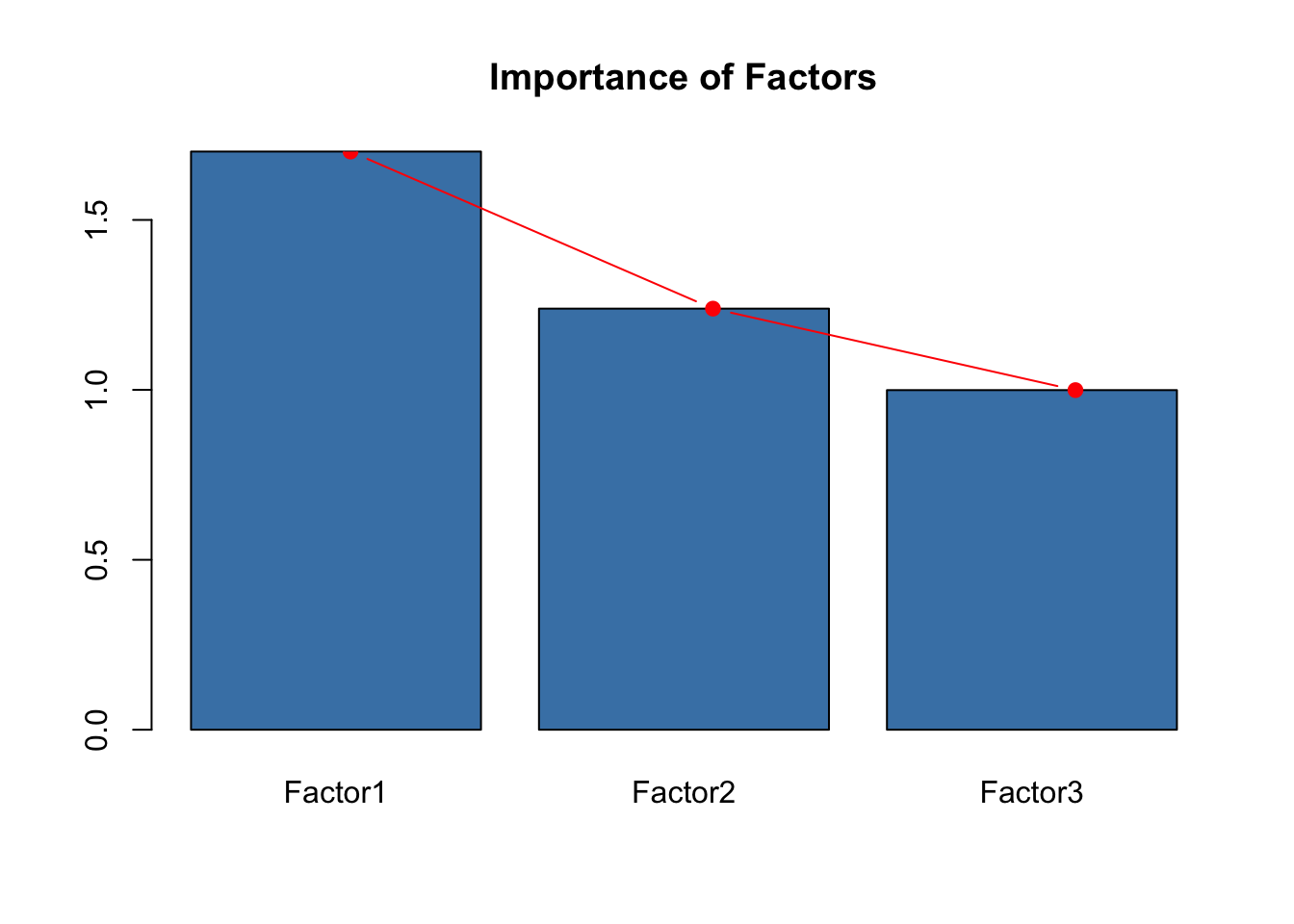
Together, the three factors explain \(56.3 \%\) of the total variance, which is a fair amount given that we’re working with a factor model rather than with PCA.
L <- life2.fa$loadingsSS <-apply(L^2, 2, sum)barplot(SS, col='steelblue' , main="Importance of Factors")lines(x =c(.75,2,3.25), SS, type="b", pch=19, col ="red")
To see how good a model at representing covariances this is, we can compute the residual matrix. This is the difference between the covariance \(\Sigma_X\) estimated by the model and the observed correlation matrix.
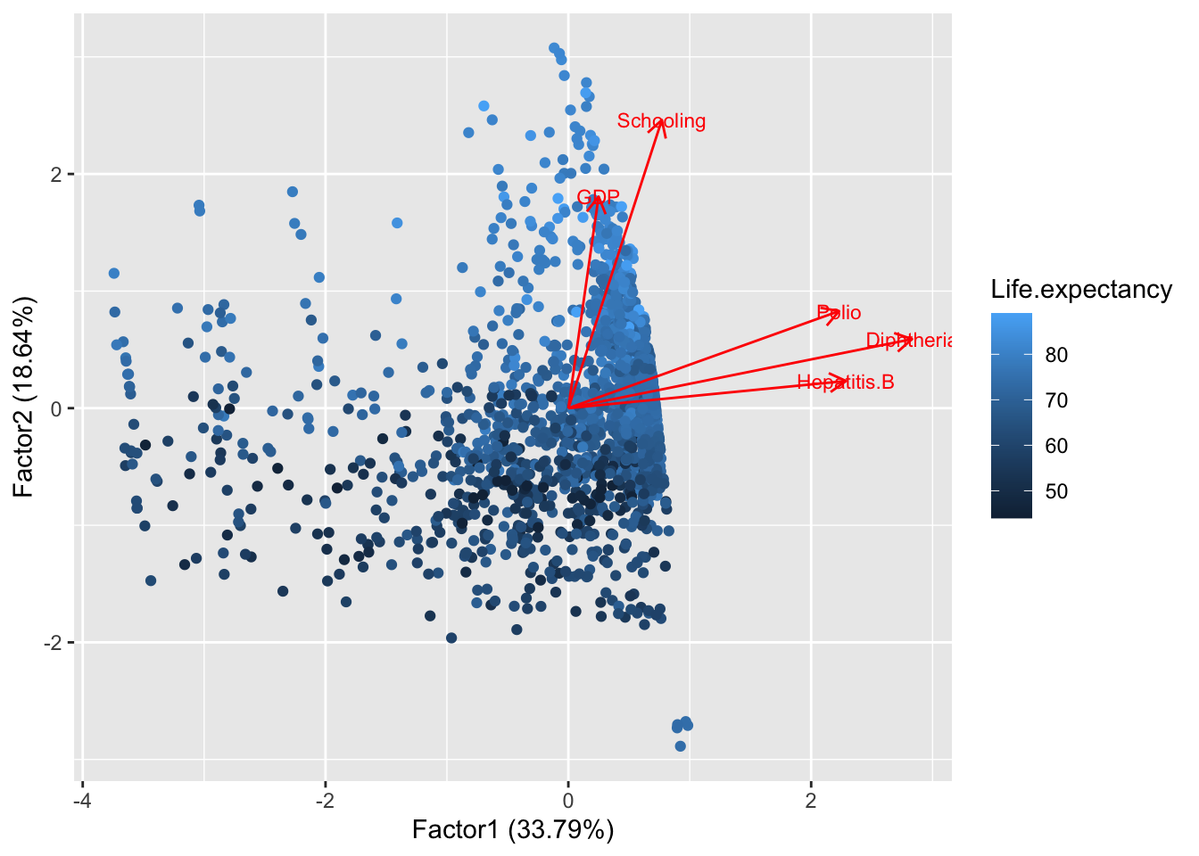
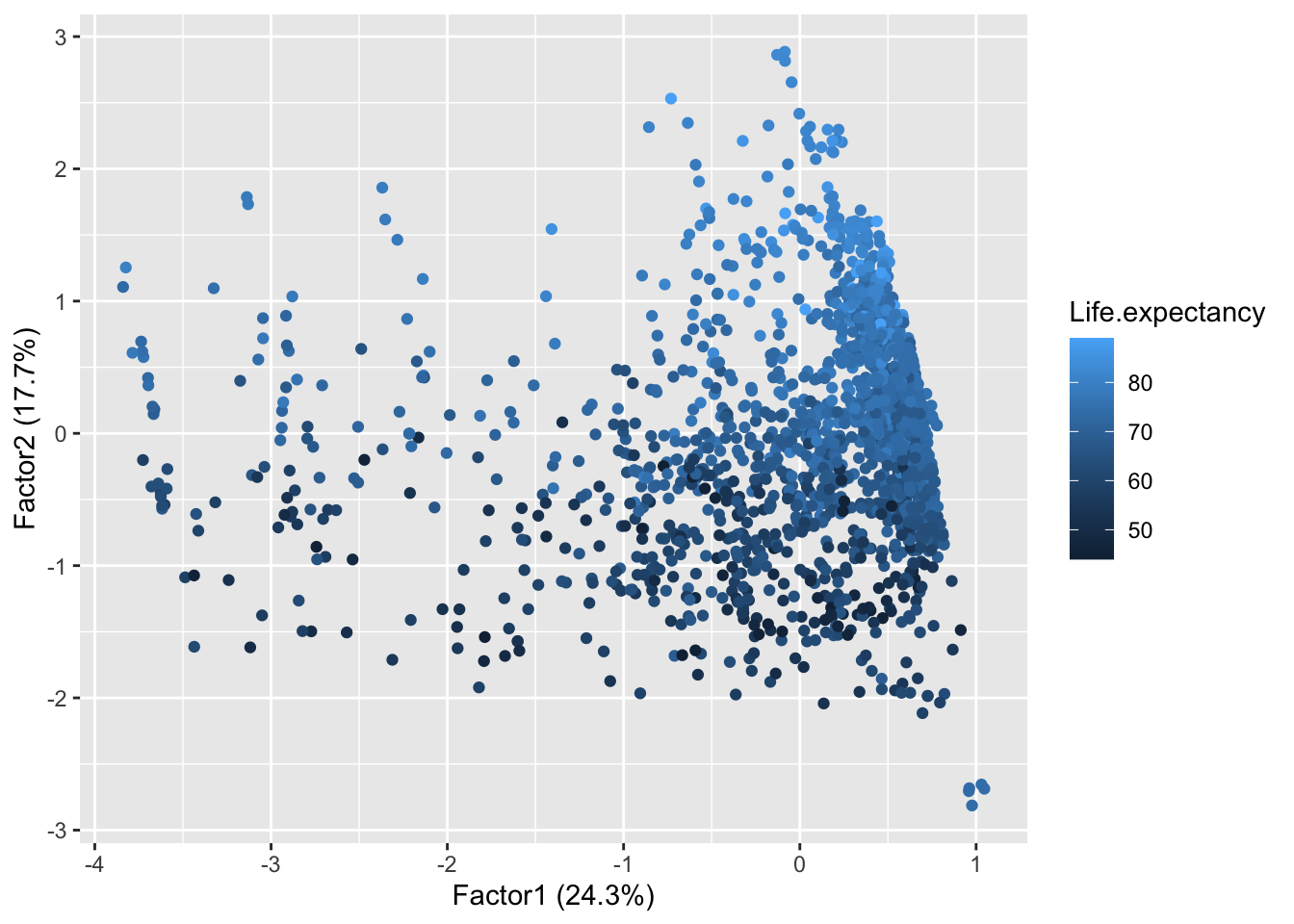
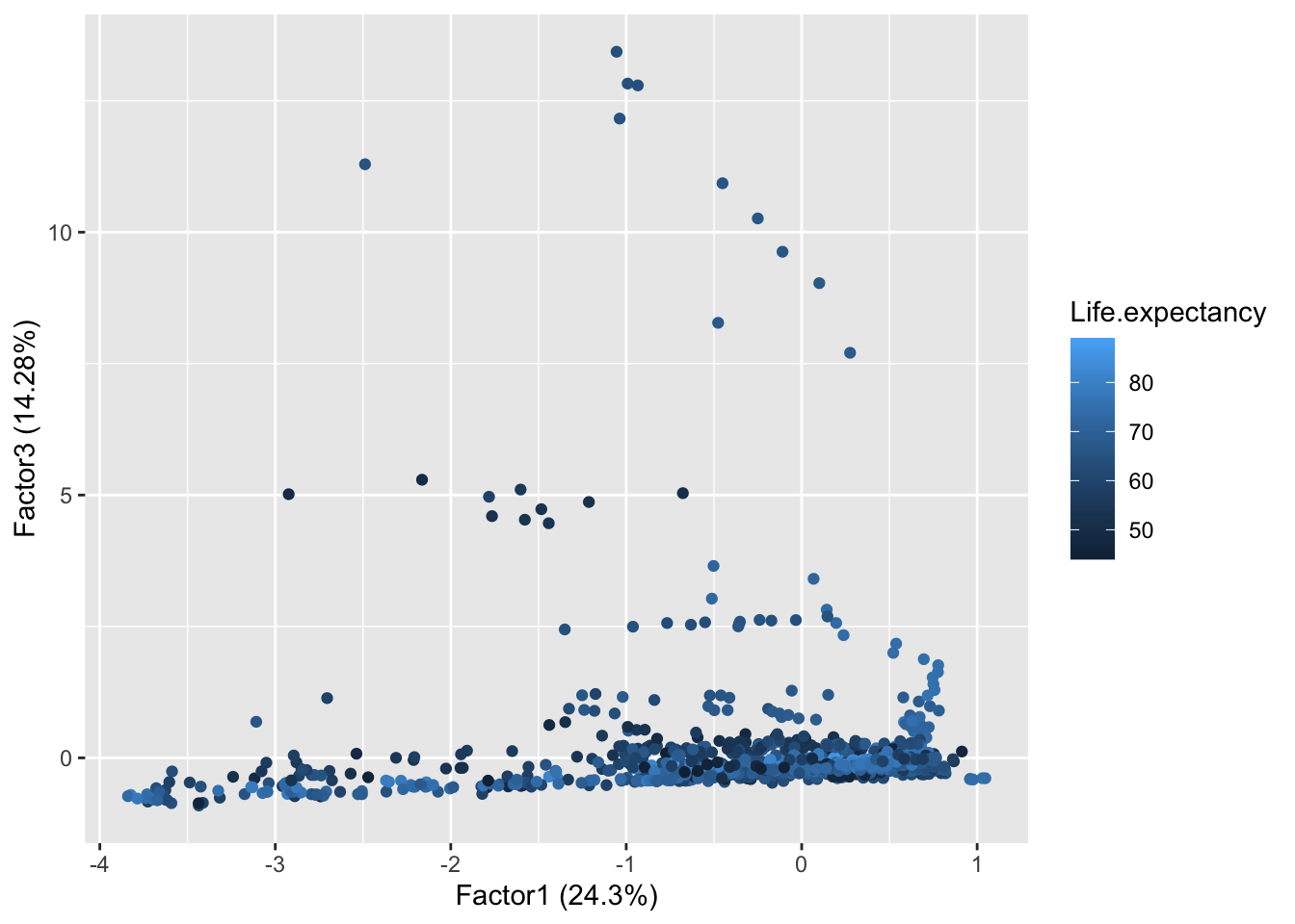
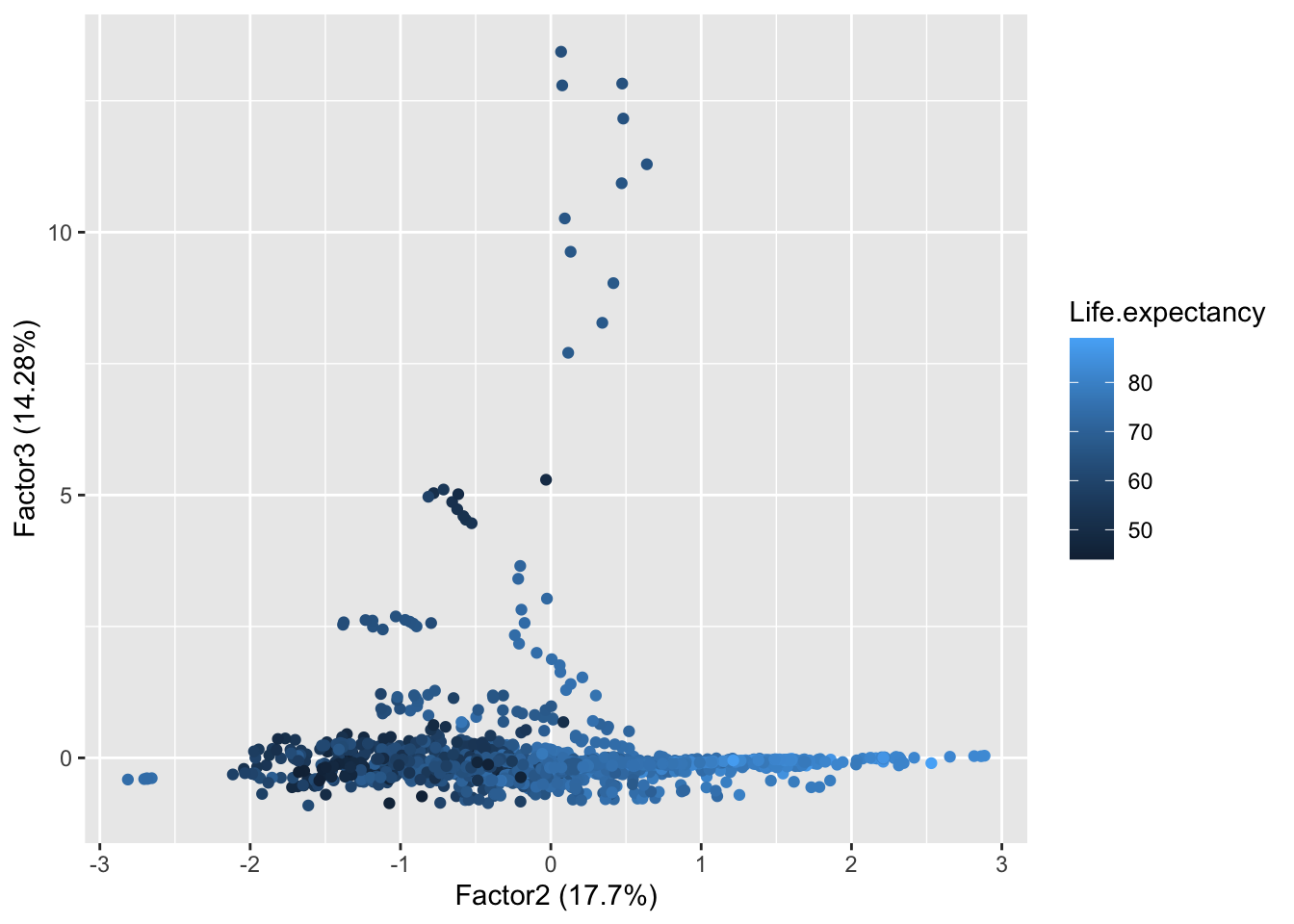
Visualization is a bit more challenging, as we have 3 factors to account for. A first method is to plot 2 factors at a time. We can do this using autoplot
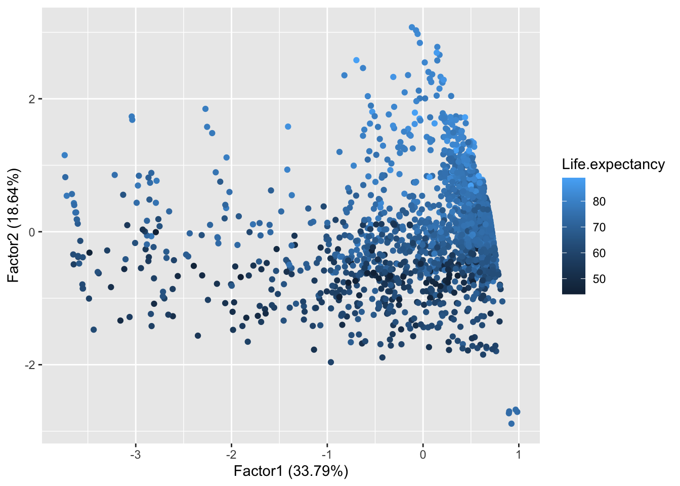
autoplot(life2.fa, data = dat, colour ='Life.expectancy')
Both factor 1 and factor 2 seem to contribute to life expectancy.
The contribution of factor 3 is less clear, as most data points are positioned low (meaning that most coutries have a low death rate for under 5).
We can still remark that even countries with low Factor3 can have a low life expectancy, meaning that Factor3 contribution alone is not very significant.
Plotting Factor 2 against Factor 3 completes the picture of the relationships between the different factors.
The following objects are masked from 'package:ggplot2':

    %+%, alpha
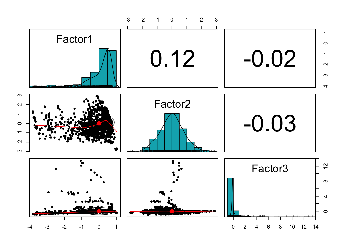
pairs.panels(life2.scores,method ="pearson", # correlation methodhist.col ="#00AFBB",density =TRUE, # show density plots )
Finally, given the greater importance of Factors 1 and 2, and the difference in scale of Factor 3, it might make sense to visualize our picture using a bubble plot, where Factor 3 is accounted on the size of the points
#installpackages('plotly')library(plotly)
Attaching package: 'plotly'
The following object is masked from 'package:ggplot2':

    last_plot
The following object is masked from 'package:stats':

    filter
The following object is masked from 'package:graphics':

    layout
The data we analyzed has a high complexity: not only it measures 11 numerical variables, but contains \(>1500\) observations! After a first exploratory analysis, we notice that there is a marked difference in behaviour between some of these observations: most notably, between the countries with high development and those with medium to low development. It seems reasonable to perform separated analysis for different kinds of countries. We begin by selecting those observations with lowest life expectancy.
Call:
factanal(x = newdat[, -c(1, 2, 3, 5, 7, 8)], factors = 3)

Uniquenesses:
  Adult.Mortality under.five.deaths       Hepatitis.B             Polio
            0.899             0.005             0.411             0.607
       Diphtheria               GDP         Schooling
            0.120             0.573             0.542

Loadings:
                  Factor1 Factor2 Factor3
Adult.Mortality                    0.311
under.five.deaths -0.168   0.981
Hepatitis.B        0.745  -0.153
Polio              0.616
Diphtheria         0.932           0.107
GDP                                0.652
Schooling          0.137           0.662

               Factor1 Factor2 Factor3
SS loadings      1.855   0.995   0.993
Proportion Var   0.265   0.142   0.142
Cumulative Var   0.265   0.407   0.549

Test of the hypothesis that 3 factors are sufficient.
The chi square statistic is 2.01 on 3 degrees of freedom.
The p-value is 0.57
What do we remark?
\(p\)-value is slightly lower: selecting less data does not improve the fitness of the model
Uniquenesses show that a good portion of variance is accounted by the model for under 5 deaths and Diphtheria immunization (as in the previous model), while the model fails to account for most of the variance of Adult mortality. Polio, GDP, and Schooling are somewhere in the middle.
The model is quite similar to the one with all data points, but now Factor 2 and Factor 3 are exchanged!
Warning: `line.width` does not currently support multiple values.
More practice 1 (French climate)
The following data set was created by researchers at Freie Universit"at in Berlin to illustrate dimension reduction techniques. It contains 36 observations of 12 variables related to climate in different locations of France. We need to preprocess it to uniformize format and treat some of the variables as numerical.
Perform FA on the data set newclim with 2 and 3 factors, and interpret uniquesnesses, loadings, and likelihood ratio test. Discuss the differences between the two models obtained. Solution to Task 1a
Click for solution
Call:
factanal(x = newclim, factors = 2, scores = "regression")

Uniquenesses:
         altitude               lat               lon            t_mean
            0.099             0.240             0.777             0.006
            t_max             t_min       relhumidity            p_mean
            0.332             0.205             0.335             0.974
         p_max24h         rainydays sun_shine_hperyrs
            0.433             0.221             0.219

Loadings:
                  Factor1 Factor2
altitude           0.159  -0.936
lat               -0.869
lon                0.472
t_mean             0.247   0.966
t_max              0.152   0.803
t_min              0.287   0.844
relhumidity       -0.815
p_mean                    -0.158
p_max24h           0.740   0.139
rainydays         -0.849  -0.242
sun_shine_hperyrs  0.879

               Factor1 Factor2
SS loadings      3.877   3.283
Proportion Var   0.352   0.298
Cumulative Var   0.352   0.651

Test of the hypothesis that 2 factors are sufficient.
The chi square statistic is 128.72 on 34 degrees of freedom.
The p-value is 6.13e-13
The likelihood ratio test indicates that the model with 2 factors is very unlikely to be accurate. This means that the analysis provided will not be sound, but it can still be valid to explore pattern in the data. Uniquenesses tell us that this model will not encode meaningfully the variance of precipitation mean and longitude, but by contrast it will encode well the variance of variables such as altitude, temperature mean, and to some extent latitude, min temperature, sunshine hours and rainy days. The cumulative variance explained by the two factors is \(65.1\%\), sufficiently high to make it worthwhile to look at this model, even though it is a hypersimplified one.
Looking at the loadings one can attempt an interpretation of the factors:
Factor 1 has positive contributions from sunshine hours and daily precipitations and negative contributions from latitude, humidity and rainy days. A labeling of this factor is challenging (see exercise 2 to see how to improve the interpretation of factors using rotations), but a fair attempt could be “general dryness”, noting that lower latitudes correspond to towns where humidity is lower, precipitations are rarer but also more substantial.
Factor 2 is somewhat easier to interpret: it is essentially a weighted measure of temperatures (altitude being negatively correlated with temperatures).
clim.fa3
Call:
factanal(x = newclim, factors = 3, scores = "regression")

Uniquenesses:
         altitude               lat               lon            t_mean
            0.075             0.005             0.608             0.005
            t_max             t_min       relhumidity            p_mean
            0.302             0.184             0.380             0.630
         p_max24h         rainydays sun_shine_hperyrs
            0.459             0.005             0.234

Loadings:
                  Factor1 Factor2 Factor3
altitude           0.207  -0.919   0.193
lat               -0.941          -0.331
lon                0.435          -0.450
t_mean             0.209   0.973
t_max              0.124   0.819   0.108
t_min              0.231   0.844  -0.224
relhumidity       -0.782
p_mean                    -0.113   0.595
p_max24h           0.706   0.182
rainydays         -0.863  -0.238   0.441
sun_shine_hperyrs  0.850   0.120  -0.169

               Factor1 Factor2 Factor3
SS loadings      3.810   3.293   1.010
Proportion Var   0.346   0.299   0.092
Cumulative Var   0.346   0.646   0.738

Test of the hypothesis that 3 factors are sufficient.
The chi square statistic is 84.32 on 25 degrees of freedom.
The p-value is 2.37e-08
With respect to the one with 2 factors, the factor analysis with 3 factors is:
More accurate (higher \(p\)-value in the likelihood ratio test) but still not very precise, so good only for exploration.
Variance of precipitation mean and longitude are better accounted for and more generally a cumulative proportion of variance of \(73.8 \%\) is explained by the model, which is very good given that we are doing FA rather than PCA.
Loadings show that Factor 1 and Factor 2 are very similar to the previous model, Factor 3 is mildly associated with “rainy weather”, where the mean precipitation and the number of rainy days count more than the maximum precipitation in 24hours. This is the kind of rain more typically associated with proximity with the ocean
Task 1b
Plot the loadings and the scores from the factor analysis with 2 factors.
Click for hint
Use autoplot() for plotting the scores, and plot()Solution to Task 1b
Click for solution
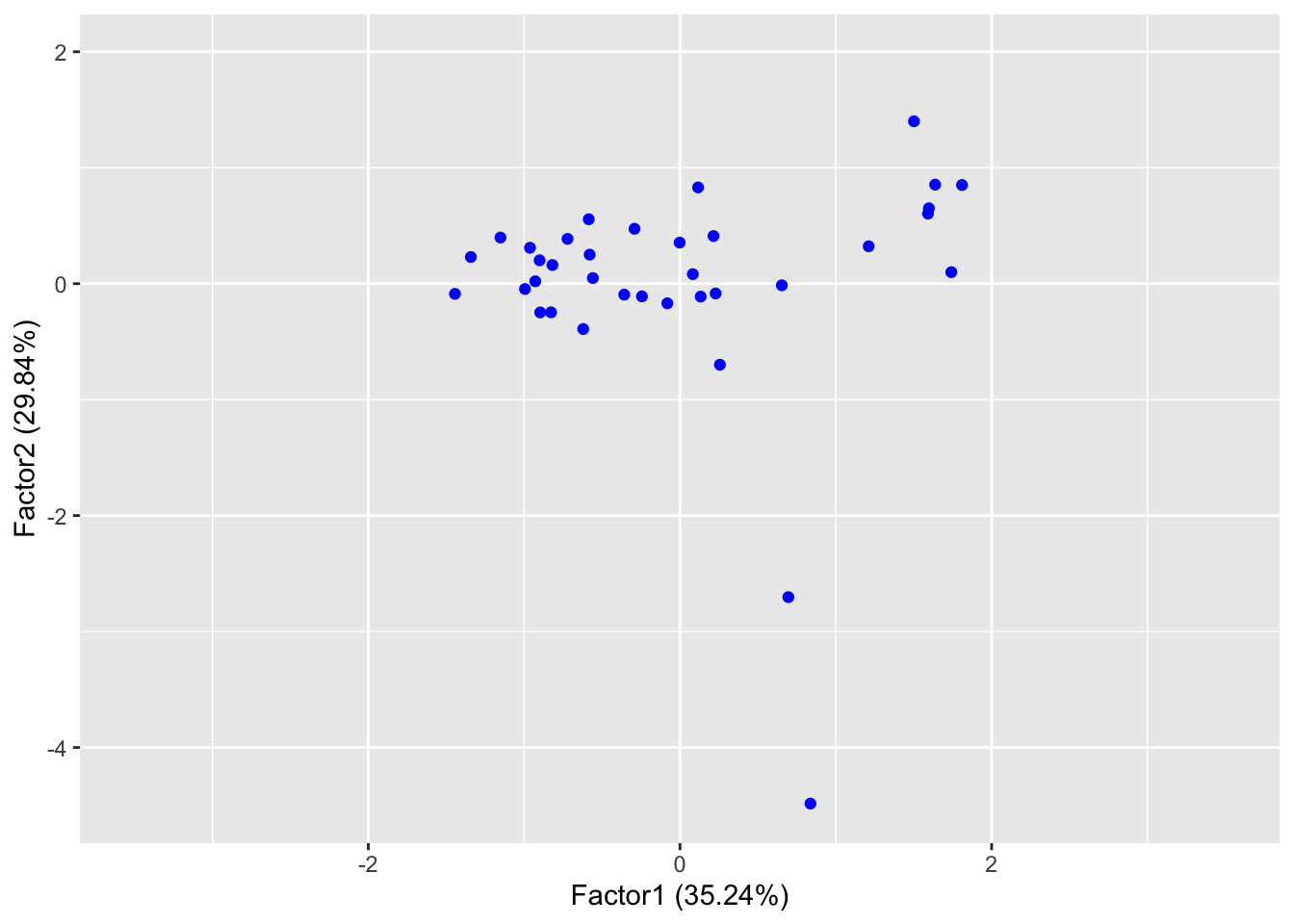
As we saw in the workshop, the scores can be plotted using the autoplot() command. Here we scale the plot to get a more faithful representation
library(ggfortify)sp <-autoplot(clim.fa2, data = clim, col="blue")sp +expand_limits(x=c(-3.5,3.5), y=c(-4.5, 2))
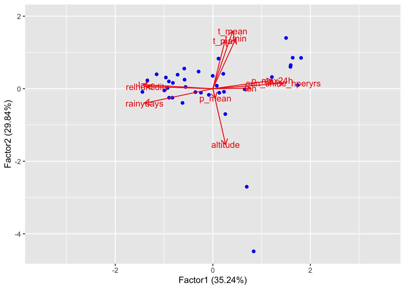
If we want to add loadings to the plot, we can do it as in the case of PCA:
It is easy to see that the variance on Factor 1 is more homogeneous, while on Factor 2 it is mostly explained by the presence of outliers. Variation in temperatures is due mostly on the altitude of the different stations, while variation in “general dryness” is a more interesting factor. We can add labels to scores to see how different locations perform:
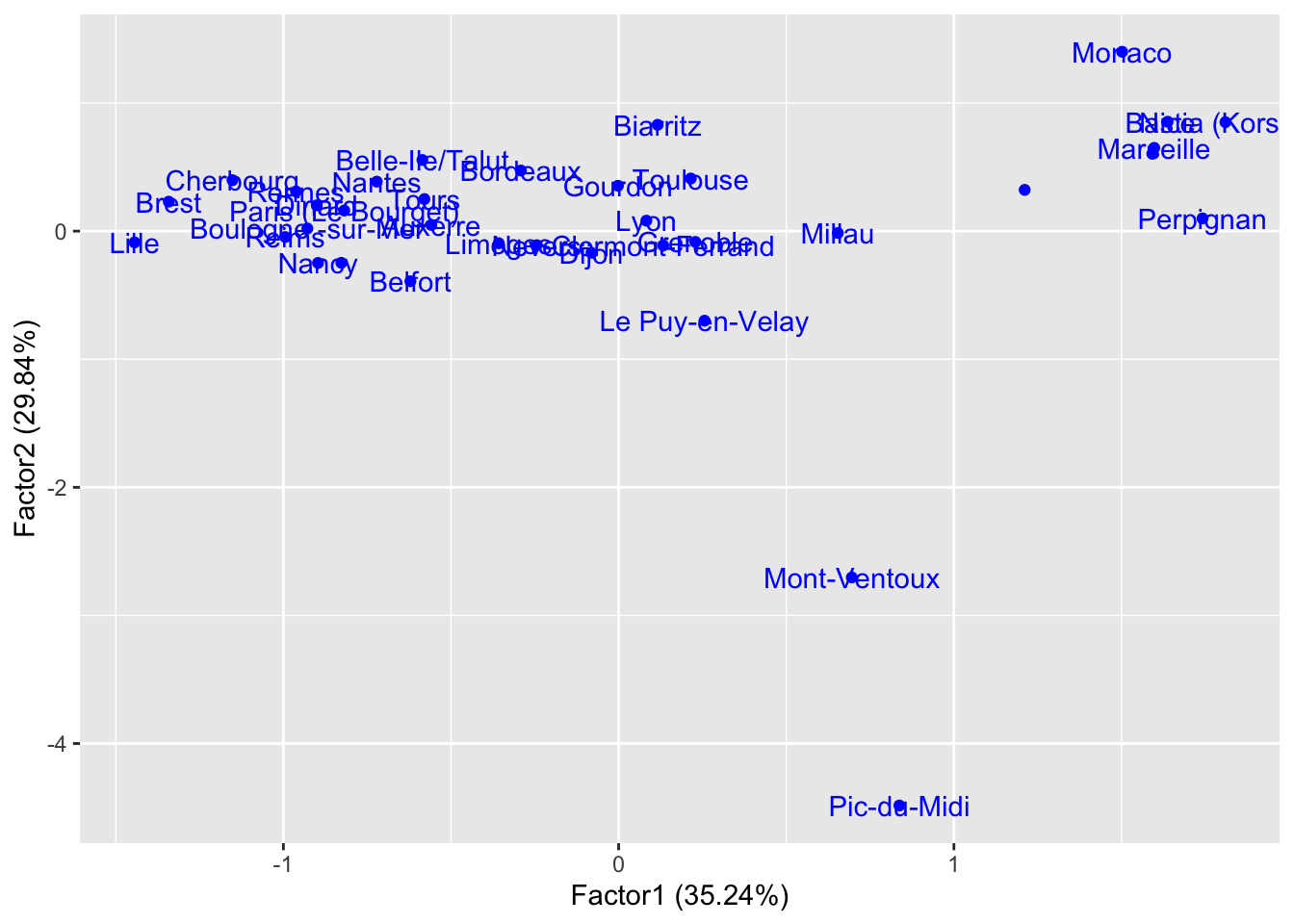
library(ggfortify)rownames(clim) <- clim$stationautoplot(clim.fa2, data = clim, col="blue", label=TRUE, repel=TRUE)
Perpignan, Marseille, and Bastia are the most generally dry, while Lille, Brest, and Cherbourg are the most generally wet. We realize in this way that Factor 1 is a very good indicator of “being next to the Mediterrenean Sea”.
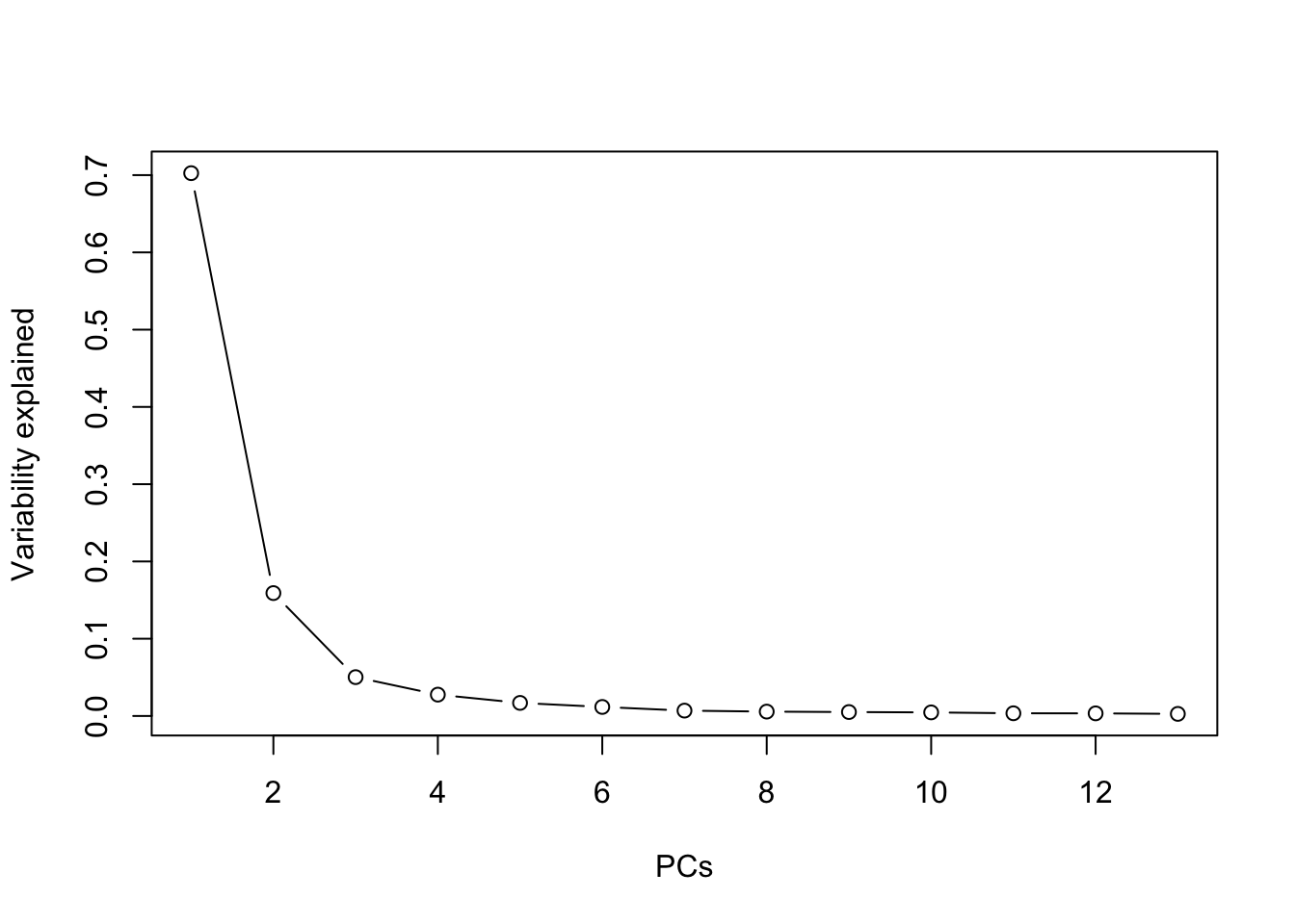
It turns out that 4 factors might be more appropriate to explain our model (see Task 3a). This can be checked with a likelihood ratio test, but also by performing PCA and checking a screeplot of the variance explained by the principal components.
Task 1c
Perform FA with 4 factors on the climate data and try to come up with a way to effectively visualize your results.
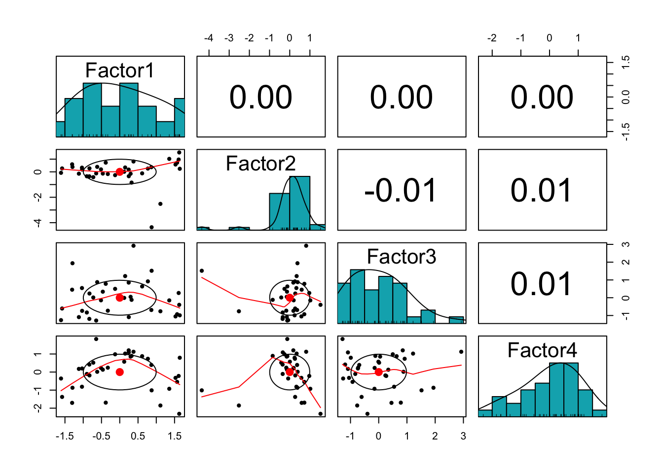
To supplement this, we can use a bubble plot, explaining two extra dimensions using colour and dimension of the bubbles. If you choose to do so, you will need to associate factors with explanating features. One idea, is to use position in the plane for those factors that are less skewed (e.g. Factor 1 in the previous plot) and non-positional features for those factors that are more skewed (e.g. Factor 2 in the previous plot).
summary(clim.fa4$scores)
    Factor1             Factor2           Factor3            Factor4
 Min.   :-1.607874   Min.   :-4.3595   Min.   :-1.28297   Min.   :-2.3126
 1st Qu.:-0.829780   1st Qu.:-0.1542   1st Qu.:-0.77915   1st Qu.:-0.6122
 Median :-0.002424   Median : 0.1886   Median :-0.06458   Median : 0.1863
 Mean   : 0.000000   Mean   : 0.0000   Mean   : 0.00000   Mean   : 0.0000
 3rd Qu.: 0.793715   3rd Qu.: 0.3855   3rd Qu.: 0.56700   3rd Qu.: 0.8086
 Max.   : 1.642677   Max.   : 1.5249   Max.   : 2.92347   Max.   : 1.8299
From this summary we see that factors 1 and 3 have similar median and mean, while for factors 2 and 4 they are quite different. We then choose to associate colour with Factor 2 and size with Factor 4.
Of course, these are not the only possibilities: other instances of scatterplot matrices, as well as parallel plots are all good choices to get more insight of your data set.
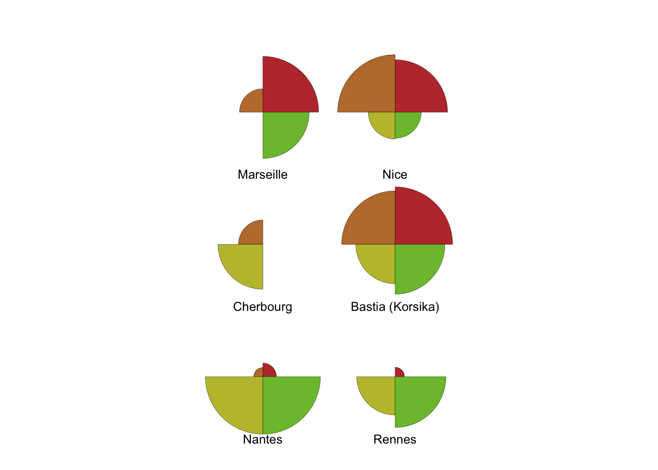
If you are interested in how particular places perform on these 4 factors you can even try out glyphs!
More practice 2 (Factor interpretation and rotation)
One aspect of Factor Analysis that we did not consider yet is that we can apply a rotation to the space of factors without changing the main features of the model: the uniquenesses will be the same, as well as the proportion of variance explained. However, rotating the space might be useful to find a better interpretation of factors. There are infinitely many way of producing a rotation: the command factanal() has built-in standard methods that allow one to easily check the most relevant ones.
Rather than using real-world data, in this exercise you’ll generate a data set from a multivariate normal distribution.
Recall from Lab2 how to generate observations of p variables from a multivariate normal distribution with correlation matrix given as \(corr(x_{i},x_{j}) = \rho^{|i-j|}\). We’ll set \(p=13\) and generate \(n=200\) observations in the case \(\rho=0.92\).
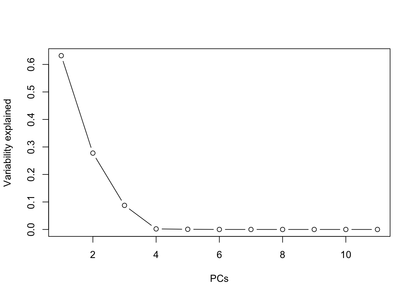
Suppose we want to perform Factor Analysis on our data set dd. Determine an appropriate number of factors to use by performing PCA. Even though the principal components are not the same in PCA and FA, the number of appropriate components in both cases is often equal, so this makes sense.
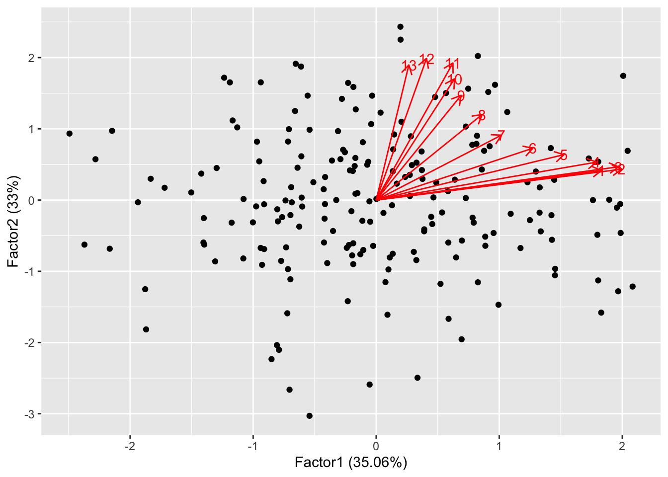
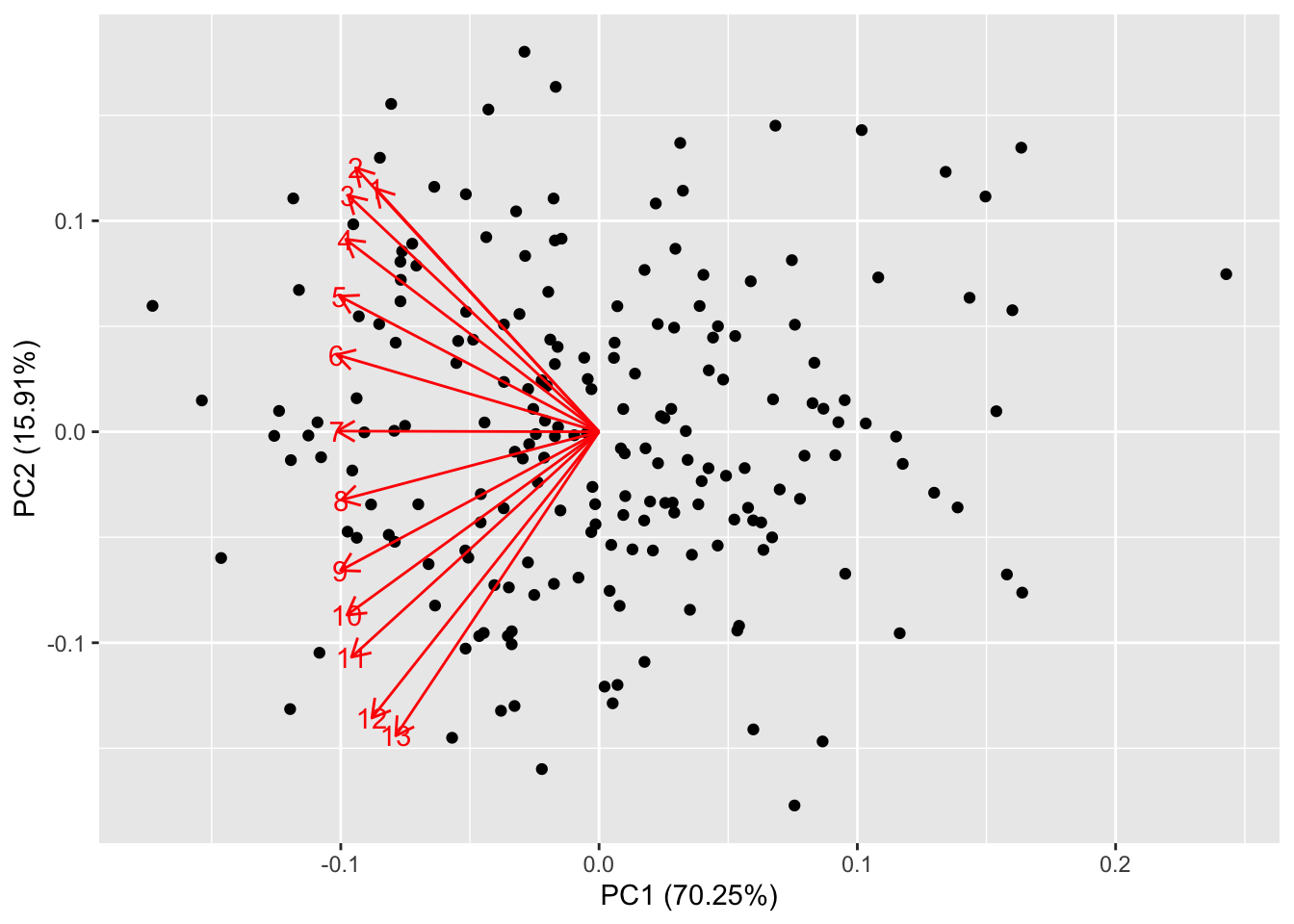
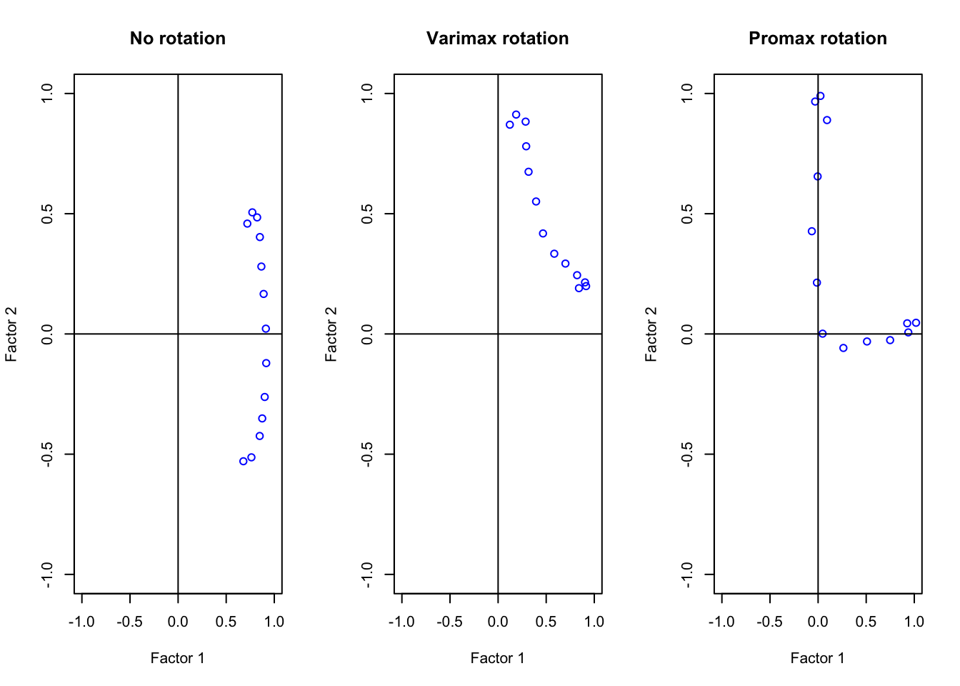
The data points are scattered quite uniformly in the space. The loadings are all in the first quadrant and are anticlockwise ordered. This is because, by design, the first few features (that are highly correlated) contribute the most to the first factor, while the last features contribute most to the second factor. This behaviour is quite similar to what happens for PCA:
autoplot(prr, loadings=TRUE, loadings.label=TRUE)
We saw that our factors are created with the aim to account for most of the variability in the data. One issue arising from this is that sometimes different factors tend to load portions of the same variables, while it would be desirable for different factors to load different variables, if possible.
The solution to this problem is to apply a rotation to the matrix of loadings. This is perfectly acceptable, as it does not affect uniquenesses and the fitness of the model. However, loadings get repositioned to help maximize interpretability. In factanal() this is controlled via the option rotation:
Compare the above rotation patterns graphically by plotting the loadings in the three situations above. Comment on which rotation gives a better interpretation of the factors
The promax rotation is clearly the best method. Our variables are either highly contributing to Factor 1 or to Factor 2 but not both! To check this, look at the factor analysis summary:
norm.fa.promax
Call:
factanal(x = dd, factors = 3, rotation = "promax")

Uniquenesses:
 [1] 0.227 0.092 0.065 0.113 0.164 0.127 0.066 0.089 0.099 0.112 0.064 0.097
[13] 0.205

Loadings:
      Factor1 Factor2 Factor3
 [1,]  0.926
 [2,]  1.018          -0.124
 [3,]  0.938
 [4,]  0.749           0.263
 [5,]  0.508           0.499
 [6,]  0.263           0.766
 [7,]                  0.931
 [8,]          0.213   0.802
 [9,]          0.427   0.646
[10,]          0.655   0.365
[11,]          0.889
[12,]          0.990
[13,]          0.967

               Factor1 Factor2 Factor3
SS loadings      3.680   3.371   3.008
Proportion Var   0.283   0.259   0.231
Cumulative Var   0.283   0.542   0.774

Factor Correlations:
        Factor1 Factor2 Factor3
Factor1   1.000  -0.694   0.717
Factor2  -0.694   1.000  -0.446
Factor3   0.717  -0.446   1.000

Test of the hypothesis that 3 factors are sufficient.
The chi square statistic is 462.16 on 42 degrees of freedom.
The p-value is 3.73e-72
With the promax rotation, the first 6 features contribute to the first factor and the last 6 contribute to the second factor. When this situation arises from real data, the interpretation of factors becomes easier.
More practice 3 (Advanced features using fa())
In this exercise, you’ll use the same climate data set of Exercise 1. This time, you’ll explore how to perform factor analysis using the fa() command.
Task 3a
Determine the number of factors you should use to perform FA.
Explore the output of fa() and compare with factanal()
Solution to task 3b
Click for solution
We first check the structure of our output:
str(clim.fa)
List of 54
 $ residual     : num [1:11, 1:11] 0.0449 -0.0453 -0.0204 0.0172 -0.0054 ...
  ..- attr(*, "dimnames")=List of 2
  .. ..$ : chr [1:11] "altitude" "lat" "lon" "t_mean" ...
  .. ..$ : chr [1:11] "altitude" "lat" "lon" "t_mean" ...
 $ dof          : num 17
 $ chi          : num 3.78
 $ nh           : num 36
 $ rms          : num 0.0309
 $ EPVAL        : num 1
 $ crms         : num 0.0556
 $ EBIC         : num -57.1
 $ ESABIC       : num -4.03
 $ fit          : num 0.978
 $ fit.off      : num 0.995
 $ sd           : num 0.0294
 $ factors      : num 4
 $ complexity   : Named num [1:11] 1.16 1.33 1.87 1.05 1.47 ...
  ..- attr(*, "names")= chr [1:11] "altitude" "lat" "lon" "t_mean" ...
 $ n.obs        : int 36
 $ objective    : num 2.2
 $ criteria     : Named num [1:3] 2.2 NA NA
  ..- attr(*, "names")= chr [1:3] "objective" "" ""
 $ STATISTIC    : num 61.2
 $ PVAL         : num 6.68e-07
 $ Call         : language fa(r = newclim, nfactors = 4)
 $ null.model   : num 13.3
 $ null.dof     : num 55
 $ null.chisq   : num 406
 $ TLI          : num 0.547
 $ CFI          : num 0.874
 $ RMSEA        : Named num [1:4] 0.267 0.201 0.348 0.9
  ..- attr(*, "names")= chr [1:4] "RMSEA" "lower" "upper" "confidence"
 $ BIC          : num 0.27
 $ SABIC        : num 53.4
 $ r.scores     : num [1:4, 1:4] 1.00 1.71e-01 -6.78e-04 7.29e-05 1.71e-01 ...
 $ R2           : num [1:4] 1.017 0.998 0.88 0.819
 $ valid        : num [1:3] 0.967 0.988 0.858
 $ score.cor    : num [1:4, 1:4] 1 0.224 -0.0146 NA 0.224 ...
 $ weights      : num [1:11, 1:4] 0.891 0.569 -0.251 0.474 0.458 ...
  ..- attr(*, "dimnames")=List of 2
  .. ..$ : chr [1:11] "altitude" "lat" "lon" "t_mean" ...
  .. ..$ : chr [1:4] "MR1" "MR2" "MR3" "MR4"
 $ rotation     : chr "oblimin"
 $ hyperplane   : Named num [1:4] 3 6 6 5
  ..- attr(*, "names")= chr [1:4] "MR1" "MR2" "MR3" "MR4"
 $ communality  : Named num [1:11] 0.955 0.782 0.405 0.982 0.865 ...
  ..- attr(*, "names")= chr [1:11] "altitude" "lat" "lon" "t_mean" ...
 $ communalities: Named num [1:11] 0.955 0.782 0.405 0.982 0.865 ...
  ..- attr(*, "names")= chr [1:11] "altitude" "lat" "lon" "t_mean" ...
 $ uniquenesses : Named num [1:11] 0.0449 0.2183 0.5945 0.0176 0.1353 ...
  ..- attr(*, "names")= chr [1:11] "altitude" "lat" "lon" "t_mean" ...
 $ values       : num [1:11] 4.543 2.828 1.063 0.566 0.245 ...
 $ e.values     : num [1:11] 4.699 2.943 1.34 0.782 0.551 ...
 $ loadings     : 'loadings' num [1:11, 1:4] 0.2523 -0.8146 0.5446 0.1292 0.0748 ...
  ..- attr(*, "dimnames")=List of 2
  .. ..$ : chr [1:11] "altitude" "lat" "lon" "t_mean" ...
  .. ..$ : chr [1:4] "MR1" "MR2" "MR3" "MR4"
 $ model        : num [1:11, 1:11] 0.9551 -0.2338 0.0101 -0.8808 -0.7662 ...
  ..- attr(*, "dimnames")=List of 2
  .. ..$ : chr [1:11] "altitude" "lat" "lon" "t_mean" ...
  .. ..$ : chr [1:11] "altitude" "lat" "lon" "t_mean" ...
 $ fm           : chr "minres"
 $ rot.mat      : num [1:4, 1:4] 0.7859 -0.6279 -0.1577 -0.0712 0.4914 ...
 $ Phi          : num [1:4, 1:4] 1 0.18294 0.05458 0.00334 0.18294 ...
  ..- attr(*, "dimnames")=List of 2
  .. ..$ : chr [1:4] "MR1" "MR2" "MR3" "MR4"
  .. ..$ : chr [1:4] "MR1" "MR2" "MR3" "MR4"
 $ Structure    : 'loadings' num [1:11, 1:4] 0.0801 -0.8145 0.5273 0.3067 0.2268 ...
  ..- attr(*, "dimnames")=List of 2
  .. ..$ : chr [1:11] "altitude" "lat" "lon" "t_mean" ...
  .. ..$ : chr [1:4] "MR1" "MR2" "MR3" "MR4"
 $ method       : chr "regression"
 $ scores       : num [1:36, 1:4] 1.581 1.524 -0.994 1.4 -0.967 ...
  ..- attr(*, "dimnames")=List of 2
  .. ..$ : NULL
  .. ..$ : chr [1:4] "MR1" "MR2" "MR3" "MR4"
 $ R2.scores    : Named num [1:4] NA 0.998 0.88 0.819
  ..- attr(*, "names")= chr [1:4] "MR1" "MR2" "MR3" "MR4"
 $ r            : num [1:11, 1:11] 1 -0.2791 -0.0103 -0.8636 -0.7716 ...
  ..- attr(*, "dimnames")=List of 2
  .. ..$ : chr [1:11] "altitude" "lat" "lon" "t_mean" ...
  .. ..$ : chr [1:11] "altitude" "lat" "lon" "t_mean" ...
 $ np.obs       : num [1:11, 1:11] 36 36 36 36 36 36 36 36 36 36 ...
  ..- attr(*, "dimnames")=List of 2
  .. ..$ : chr [1:11] "altitude" "lat" "lon" "t_mean" ...
  .. ..$ : chr [1:11] "altitude" "lat" "lon" "t_mean" ...
 $ fn           : chr "fa"
 $ Vaccounted   : num [1:5, 1:4] 3.986 0.362 0.362 0.443 0.443 ...
  ..- attr(*, "dimnames")=List of 2
  .. ..$ : chr [1:5] "SS loadings" "Proportion Var" "Cumulative Var" "Proportion Explained" ...
  .. ..$ : chr [1:4] "MR1" "MR2" "MR3" "MR4"
 $ ECV          : Named num [1:4] 0.443 0.81 0.935 1
  ..- attr(*, "names")= chr [1:4] "MR1" "MR2" "MR3" "MR4"
 - attr(*, "class")= chr [1:2] "psych" "fa"
Clearly, fa() is a more sophisticated function, containing 52 types of output. But don’t worry, you are not supposed to know all of them! We distinguish, among others, many concepts that we explored so far: the uniquenesses, the loadings, the communality, the residuals and rot.mat, which stands for rotation matrix.
To view the results of the analysis, we can use the print() command:
print(clim.fa)
Factor Analysis using method =  minres
Call: fa(r = newclim, nfactors = 4)
Standardized loadings (pattern matrix) based upon correlation matrix
                    MR1   MR2   MR3   MR4   h2    u2 com
altitude           0.25 -0.97  0.10  0.01 0.96 0.045 1.2
lat               -0.81  0.09 -0.32  0.03 0.78 0.218 1.3
lon                0.54 -0.02 -0.25 -0.25 0.41 0.595 1.9
t_mean             0.13  0.96  0.04  0.06 0.98 0.018 1.0
t_max              0.07  0.84 -0.02 -0.41 0.86 0.135 1.5
t_min              0.18  0.79  0.05  0.38 0.90 0.101 1.6
relhumidity       -0.87  0.07  0.07  0.33 0.85 0.148 1.3
p_mean            -0.07 -0.04  0.86  0.02 0.74 0.256 1.0
p_max24h           0.71  0.17  0.37 -0.08 0.73 0.269 1.7
rainydays         -0.92 -0.12  0.26 -0.18 0.97 0.026 1.3
sun_shine_hperyrs  0.87  0.01 -0.02  0.22 0.81 0.189 1.1

                       MR1  MR2  MR3  MR4
SS loadings           3.99 3.30 1.13 0.59
Proportion Var        0.36 0.30 0.10 0.05
Cumulative Var        0.36 0.66 0.76 0.82
Proportion Explained  0.44 0.37 0.13 0.07
Cumulative Proportion 0.44 0.81 0.93 1.00

 With factor correlations of
     MR1   MR2   MR3  MR4
MR1 1.00  0.18  0.05 0.00
MR2 0.18  1.00 -0.14 0.07
MR3 0.05 -0.14  1.00 0.01
MR4 0.00  0.07  0.01 1.00

Mean item complexity =  1.3
Test of the hypothesis that 4 factors are sufficient.

df null model =  55  with the objective function =  13.31 with Chi Square =  406.03
df of  the model are 17  and the objective function was  2.2

The root mean square of the residuals (RMSR) is  0.03
The df corrected root mean square of the residuals is  0.06

The harmonic n.obs is  36 with the empirical chi square  3.78  with prob <  1
The total n.obs was  36  with Likelihood Chi Square =  61.19  with prob <  6.7e-07

Tucker Lewis Index of factoring reliability =  0.547
RMSEA index =  0.267  and the 90 % confidence intervals are  0.201 0.348
BIC =  0.27
Fit based upon off diagonal values = 1
This is a lot to digest! But we can recognize some familiar quantities: the loadings, uniquenesses and communalities. The results agree with those of Exercise 1.