Principal Component Analysis

Unsupervised learning

The main two types of statistical learning are: * Supervised learning, which is “learning with a teacher”: the student present an estimate response for each observation, the teacher provides the correct answer and the student improves their models. * Unsupervised learning, which is “learning without a teacher”. In this respect, it is more challenging (no training, no validation, no simple goal). But sometimes you can’t avoid using it!

Unsupervised learning is often overlooked, but it has many applications: recommender systems, document search, fake image analysis, risk management, …

Dimensionality Reduction

Dimensionality reduction methods aim to reduce the number of variables, retaining much of the properties of the original data. They are used to * Improve storage and computational complexity * Prevent overfitting in data analysis * Reduce noise and detecting anomalies The most important technique for dimensionality reduction is principal component analysis (PCA).

For a description of how to define the principal components and the related quantities, please refer to the slides or to the very readable chapter 12 of An introduction to statistical learning (by James, Witten, Hastie and Tibshirani).

Here below, we discuss how to use PCA for dimensionality reduction.

Proportion of variance

We want to establish a technique to select the more relevant \(PC_k\), to minimize loss of information when we reduce the dimension. So our main question is how to measure the amount of structure captured by each \(PC_k\).

The proportion of variance is what we need to use here. Recall that the variance explained by \(\phi_k\) is

[_k = _k^T _k,]

which is exactly the \(k\)-th eigenvalue of \(\mathbf{\Sigma}\).

The proportion of variance explained by \(\phi_k\) is then

[ .]

A good dimension reduction technique must retain at least 80% of the original variance, as a rule of thumb. In some situations, this might be replaced by elbow rule.

Possible issues

The procedure always works well in theory, but presents some issues when looking at data in real life.

  • If the original variables are highly uncorrelated, we need too many principal components to explain at least 80% of variance

  • By changing units of measurement, the variances also change, for the very same data!

  • Even when the units are the same, the standard deviation of the original variables can vary a lot (e.g. Iris data): the variables with higher standard deviation will be more represented in the first PCs.

Issue 1 is structural, so no solution can be found. Issues 2 and 3 can be solved by scaling the data set.

Scaling the original data

Let \(\mathbf{X}\) be the matrix of a data set. Scaling \(\mathbf{X}\) means replacing each column \(\mathbf{X}\) of \(\mathbf{X}\) with

[ ,] where \(\mathbf{\mu} = \begin{pmatrix} \mu \\ \mu\\ \vdots \\ \mu \end{pmatrix}\) is the mean vector of \(\mathbf{X}\) and \(sd\) is the standard deviation of \(\mathbf{X}\).

The covariance matrix of the scaled data is called the correlation matrix of the original data.

Other relevant notions for PCA are:

  • Correlation between PC and original variables: these are obtained as dot products of the loadings against the PCs
  • Quality of representation (cos2):
  • Absolute contributions (contrib):

PCA using prcomp()

Now that we are backed by the theory, let’s explore once again how to perform PCA with R. We will analyze the US Senate data sets, reduce its dimension in an appropriate way and see what this analysis tells us about the evolution of political parties in the US.

Us Senate data

You can download the data sets from Blackboard as .csv files.

We first start by loading the datasets in our environment together with the libraries.

#install.packages("factoextra")
library(factoextra)
Loading required package: ggplot2
Welcome! Want to learn more? See two factoextra-related books at https://goo.gl/ve3WBa
library(dplyr)

Attaching package: 'dplyr'
The following objects are masked from 'package:stats':

    filter, lag
The following objects are masked from 'package:base':

    intersect, setdiff, setequal, union
data07 <- read.csv("senate-2007.csv")
data17 <- read.csv("senate-2017.csv")

We then select only the numeric features:

data07N <- data07 %>%
  select_if(is.numeric)
data17N <- data17 %>%
  select_if(is.numeric)

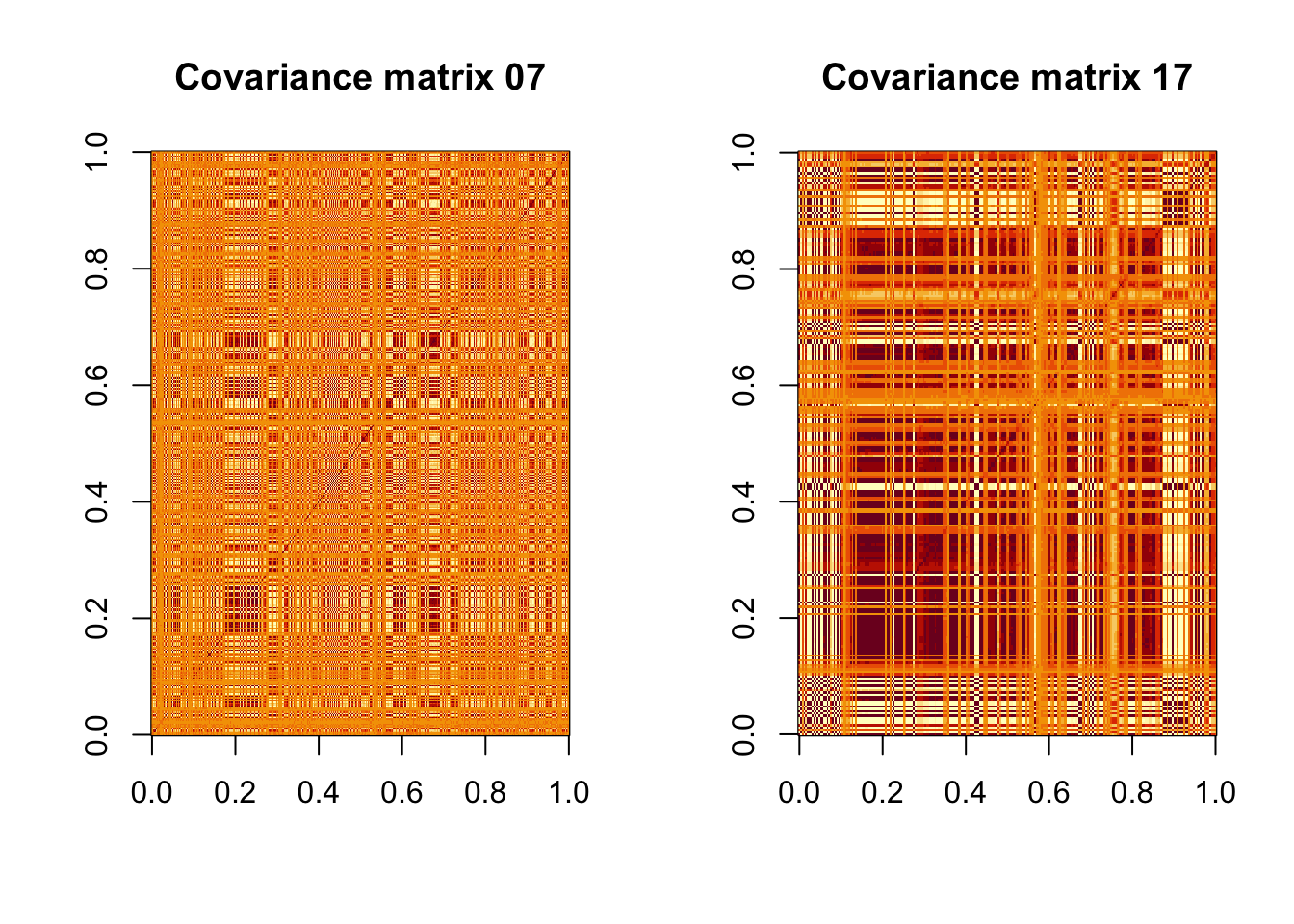
First of all, note that you can’t check the correlation matrix from a plot matrix, as it is just too big! We can try to visualize the matrix with a color plot:

Sigma07 <- cov(data07N)
Sigma17 <- cov(data17N)
par(mfrow=c(1, 2))
image(t(Sigma07), main = "Covariance matrix 07")
image(t(Sigma17), main = "Covariance matrix 17")

There is at least some redundancy in the data, which makes it worthwhile to try PCA. In the second plot this is more evident, so we might guess that PCA will be even more effective there.

/ Let us get the principal components using prcomp(). There is an argument to be made in favor of not to scaling the data: high variance in an observation means a higher level of disagreement in senators votes, while low variance means that most of them voted in the same way. If we care more about those issues that are more debated (e.g. gun laws) and less about those on which everyone agrees (e.g. raising senators’ salary) then it is preferable not to scale the data.

pr.out07 <- prcomp(data07N)
pr.out17 <- prcomp(data17N)

The output contains many objects

names(pr.out07)
[1] "sdev"     "rotation" "center"   "scale"    "x"       

We can check now the importance of principal components in the two cases

summary(pr.out07)
Importance of components:
                           PC1     PC2     PC3    PC4     PC5    PC6     PC7
Standard deviation     12.9042 3.71408 3.03882 2.4098 2.19140 2.0549 1.91235
Proportion of Variance  0.5562 0.04607 0.03084 0.0194 0.01604 0.0141 0.01221
Cumulative Proportion   0.5562 0.60225 0.63310 0.6525 0.66853 0.6826 0.69485
                           PC8     PC9    PC10   PC11    PC12    PC13    PC14
Standard deviation     1.81034 1.79620 1.77976 1.7214 1.67003 1.60616 1.56163
Proportion of Variance 0.01095 0.01078 0.01058 0.0099 0.00932 0.00862 0.00815
Cumulative Proportion  0.70580 0.71657 0.72715 0.7370 0.74637 0.75498 0.76313
                          PC15    PC16    PC17    PC18   PC19    PC20    PC21
Standard deviation     1.53252 1.51194 1.48791 1.47152 1.4476 1.40269 1.39002
Proportion of Variance 0.00784 0.00764 0.00739 0.00723 0.0070 0.00657 0.00645
Cumulative Proportion  0.77097 0.77861 0.78600 0.79324 0.8002 0.80681 0.81326
                          PC22    PC23    PC24    PC25    PC26   PC27    PC28
Standard deviation     1.35985 1.32609 1.32011 1.28057 1.27026 1.2595 1.22948
Proportion of Variance 0.00618 0.00587 0.00582 0.00548 0.00539 0.0053 0.00505
Cumulative Proportion  0.81944 0.82531 0.83113 0.83661 0.84200 0.8473 0.85234
                          PC29    PC30    PC31    PC32    PC33    PC34    PC35
Standard deviation     1.22124 1.21861 1.19118 1.16494 1.14058 1.12554 1.10577
Proportion of Variance 0.00498 0.00496 0.00474 0.00453 0.00435 0.00423 0.00408
Cumulative Proportion  0.85733 0.86229 0.86703 0.87156 0.87590 0.88013 0.88422
                          PC36    PC37    PC38    PC39   PC40    PC41    PC42
Standard deviation     1.09615 1.07222 1.06166 1.04658 1.0378 1.02996 1.00640
Proportion of Variance 0.00401 0.00384 0.00376 0.00366 0.0036 0.00354 0.00338
Cumulative Proportion  0.88823 0.89207 0.89584 0.89949 0.9031 0.90664 0.91002
                          PC43    PC44    PC45    PC46    PC47    PC48    PC49
Standard deviation     0.99843 0.98258 0.98042 0.96616 0.95144 0.94407 0.91291
Proportion of Variance 0.00333 0.00322 0.00321 0.00312 0.00302 0.00298 0.00278
Cumulative Proportion  0.91335 0.91657 0.91978 0.92290 0.92592 0.92890 0.93168
                          PC50    PC51    PC52    PC53    PC54    PC55    PC56
Standard deviation     0.90311 0.89371 0.87048 0.86888 0.85340 0.84171 0.82562
Proportion of Variance 0.00272 0.00267 0.00253 0.00252 0.00243 0.00237 0.00228
Cumulative Proportion  0.93441 0.93708 0.93961 0.94213 0.94456 0.94693 0.94920
                          PC57    PC58    PC59    PC60   PC61    PC62   PC63
Standard deviation     0.82342 0.81051 0.80683 0.79840 0.7925 0.77049 0.7552
Proportion of Variance 0.00226 0.00219 0.00217 0.00213 0.0021 0.00198 0.0019
Cumulative Proportion  0.95147 0.95366 0.95584 0.95797 0.9601 0.96205 0.9639
                          PC64    PC65    PC66    PC67    PC68    PC69    PC70
Standard deviation     0.74195 0.73172 0.72879 0.70627 0.70032 0.68822 0.67301
Proportion of Variance 0.00184 0.00179 0.00177 0.00167 0.00164 0.00158 0.00151
Cumulative Proportion  0.96579 0.96758 0.96935 0.97102 0.97266 0.97424 0.97575
                         PC71   PC72   PC73    PC74    PC75    PC76    PC77
Standard deviation     0.6712 0.6699 0.6478 0.63796 0.63142 0.61631 0.61038
Proportion of Variance 0.0015 0.0015 0.0014 0.00136 0.00133 0.00127 0.00124
Cumulative Proportion  0.9773 0.9788 0.9802 0.98152 0.98285 0.98412 0.98536
                          PC78    PC79    PC80   PC81    PC82    PC83    PC84
Standard deviation     0.59675 0.58376 0.56136 0.5481 0.53674 0.52440 0.51468
Proportion of Variance 0.00119 0.00114 0.00105 0.0010 0.00096 0.00092 0.00088
Cumulative Proportion  0.98655 0.98769 0.98874 0.9898 0.99071 0.99163 0.99251
                          PC85   PC86    PC87    PC88    PC89    PC90    PC91
Standard deviation     0.50177 0.4885 0.48019 0.45426 0.43499 0.43203 0.40844
Proportion of Variance 0.00084 0.0008 0.00077 0.00069 0.00063 0.00062 0.00056
Cumulative Proportion  0.99335 0.9941 0.99492 0.99561 0.99624 0.99686 0.99742
                          PC92    PC93    PC94    PC95    PC96    PC97    PC98
Standard deviation     0.39534 0.36208 0.35420 0.31679 0.31342 0.29432 0.27198
Proportion of Variance 0.00052 0.00044 0.00042 0.00034 0.00033 0.00029 0.00025
Cumulative Proportion  0.99794 0.99838 0.99880 0.99914 0.99946 0.99975 1.00000
                           PC99
Standard deviation     1.36e-14
Proportion of Variance 0.00e+00
Cumulative Proportion  1.00e+00
summary(pr.out17)
Importance of components:
                           PC1    PC2     PC3     PC4     PC5    PC6     PC7
Standard deviation     12.0503 2.9027 1.82664 1.70235 1.29058 1.2370 1.19967
Proportion of Variance  0.7686 0.0446 0.01766 0.01534 0.00882 0.0081 0.00762
Cumulative Proportion   0.7686 0.8132 0.83089 0.84623 0.85505 0.8631 0.87077
                           PC8     PC9    PC10    PC11    PC12    PC13    PC14
Standard deviation     1.11374 1.07762 1.05381 1.03398 1.01148 0.95085 0.91687
Proportion of Variance 0.00657 0.00615 0.00588 0.00566 0.00542 0.00479 0.00445
Cumulative Proportion  0.87733 0.88348 0.88936 0.89502 0.90043 0.90522 0.90967
                          PC15    PC16    PC17    PC18    PC19   PC20    PC21
Standard deviation     0.89851 0.86111 0.84270 0.81861 0.81776 0.7896 0.77534
Proportion of Variance 0.00427 0.00393 0.00376 0.00355 0.00354 0.0033 0.00318
Cumulative Proportion  0.91394 0.91787 0.92163 0.92517 0.92871 0.9320 0.93520
                         PC22    PC23    PC24    PC25    PC26    PC27    PC28
Standard deviation     0.7404 0.73203 0.71876 0.70269 0.67188 0.65235 0.64574
Proportion of Variance 0.0029 0.00284 0.00273 0.00261 0.00239 0.00225 0.00221
Cumulative Proportion  0.9381 0.94093 0.94367 0.94628 0.94867 0.95092 0.95313
                          PC29    PC30    PC31    PC32   PC33    PC34    PC35
Standard deviation     0.63316 0.62168 0.60849 0.60280 0.5667 0.56380 0.55342
Proportion of Variance 0.00212 0.00205 0.00196 0.00192 0.0017 0.00168 0.00162
Cumulative Proportion  0.95525 0.95730 0.95926 0.96118 0.9629 0.96456 0.96619
                          PC36   PC37    PC38    PC39    PC40    PC41    PC42
Standard deviation     0.55231 0.5329 0.52293 0.51992 0.50170 0.49733 0.48640
Proportion of Variance 0.00161 0.0015 0.00145 0.00143 0.00133 0.00131 0.00125
Cumulative Proportion  0.96780 0.9693 0.97075 0.97218 0.97351 0.97482 0.97608
                          PC43    PC44    PC45    PC46    PC47    PC48    PC49
Standard deviation     0.48504 0.48082 0.46988 0.46212 0.44674 0.43645 0.43040
Proportion of Variance 0.00125 0.00122 0.00117 0.00113 0.00106 0.00101 0.00098
Cumulative Proportion  0.97732 0.97855 0.97971 0.98084 0.98190 0.98291 0.98389
                          PC50    PC51    PC52   PC53    PC54    PC55    PC56
Standard deviation     0.41828 0.40480 0.39884 0.3895 0.38140 0.37360 0.36564
Proportion of Variance 0.00093 0.00087 0.00084 0.0008 0.00077 0.00074 0.00071
Cumulative Proportion  0.98482 0.98568 0.98652 0.9873 0.98810 0.98884 0.98954
                          PC57    PC58    PC59    PC60    PC61    PC62    PC63
Standard deviation     0.35721 0.35284 0.34250 0.32554 0.32372 0.32072 0.30358
Proportion of Variance 0.00068 0.00066 0.00062 0.00056 0.00055 0.00054 0.00049
Cumulative Proportion  0.99022 0.99088 0.99150 0.99206 0.99262 0.99316 0.99365
                          PC64    PC65    PC66    PC67    PC68    PC69    PC70
Standard deviation     0.30149 0.28769 0.28589 0.27252 0.26746 0.25620 0.25116
Proportion of Variance 0.00048 0.00044 0.00043 0.00039 0.00038 0.00035 0.00033
Cumulative Proportion  0.99413 0.99457 0.99500 0.99539 0.99577 0.99612 0.99645
                          PC71   PC72    PC73    PC74    PC75    PC76   PC77
Standard deviation     0.24160 0.2385 0.22971 0.21421 0.20824 0.20091 0.1944
Proportion of Variance 0.00031 0.0003 0.00028 0.00024 0.00023 0.00021 0.0002
Cumulative Proportion  0.99676 0.9971 0.99734 0.99759 0.99781 0.99803 0.9982
                          PC78    PC79    PC80    PC81    PC82    PC83    PC84
Standard deviation     0.19135 0.18550 0.17552 0.16872 0.16317 0.15708 0.14630
Proportion of Variance 0.00019 0.00018 0.00016 0.00015 0.00014 0.00013 0.00011
Cumulative Proportion  0.99842 0.99860 0.99877 0.99892 0.99906 0.99919 0.99930
                          PC85   PC86    PC87    PC88    PC89    PC90    PC91
Standard deviation     0.14214 0.1355 0.12813 0.12415 0.11872 0.10075 0.09239
Proportion of Variance 0.00011 0.0001 0.00009 0.00008 0.00007 0.00005 0.00005
Cumulative Proportion  0.99941 0.9995 0.99959 0.99968 0.99975 0.99980 0.99985
                          PC92    PC93    PC94    PC95    PC96    PC97
Standard deviation     0.08683 0.07978 0.07389 0.06650 0.05529 0.04076
Proportion of Variance 0.00004 0.00003 0.00003 0.00002 0.00002 0.00001
Cumulative Proportion  0.99989 0.99992 0.99995 0.99998 0.99999 1.00000
                            PC98      PC99
Standard deviation     1.156e-14 1.105e-15
Proportion of Variance 0.000e+00 0.000e+00
Cumulative Proportion  1.000e+00 1.000e+00

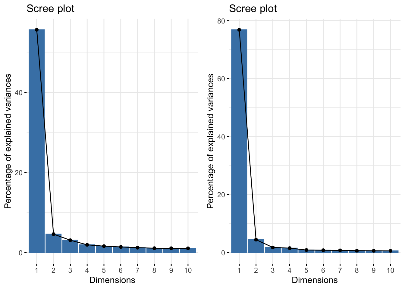
In the first case, one needs 19 principal components to capture \(\geq 80\%\) of variance, in the second case, it is sufficient to retain two of them! This is particularly striking, as our original set of variables contains more than 250 items! In both cases, \(PC1\) captures a lot of variance, so it is something interesting to look at.

To convince ourselves of this, we can make a screeplot

require(gridExtra)
Loading required package: gridExtra

Attaching package: 'gridExtra'
The following object is masked from 'package:dplyr':

    combine
plot1 <- fviz_eig(pr.out07)
plot2 <- fviz_eig(pr.out17)
grid.arrange(plot1, plot2, ncol=2)

Note that, even in the first case, there is a big discrepancy between PC1 and the other principal components. In this case one can make an exception to the “80% rule” by noticing two things:

  • Original variables are a lot.
  • There is a clear elbow in the screeplot: this is the point where the edges begin to flatten, and it occurs right after PC1.

According to this elbow method, we can make an argument for retaining only the first principal component.

Even when only one principal component is deemed to be sufficient, it is worthwhile to visualize scores on a biplot, that can be slightly squeezed on the horizontal axis, if needed.

plot1 <- fviz_pca_ind(pr.out07, label=FALSE)
plot2 <- fviz_pca_ind(pr.out17, label=FALSE)
grid.arrange(plot1, plot2, ncol=2)

We see a clear divide between senators on the left and on the right of the principal component. What could this represent?

plot1 <- fviz_pca_ind(pr.out07, col.ind = data07$Party, label=FALSE)
plot2 <- fviz_pca_ind(pr.out17, col.ind = data17$Party, label=FALSE)
grid.arrange(plot1, plot2, ncol=2)

The first principal component is a very good representation of party affiliation! From the historic comparison of the two plots, we can see that the divide between Democrats and Republicans has grown a lot between 2007 and 2017, this is an indication that polarization of senators along party lines is a phenomenon that predates the election of Donald Trump (2016).