Practical 5 - Principal Component Analysis

This computer practical consists of three exercises.

• In exercise 1, you will use factoextra package to extract more information and visualise the results obtained by principal component analysis on the USArrests dataset;
• In exercise 2, you will examine how the strength of existing redundancy in data affects the PCA results;
• In exercise 3, you will get a taste of principal component regression.

Exercise 1 (factoextra)

First load the following package into your workspace for visualisation.

library(factoextra)

In this first part, you will analyze data from the database USArrests, which is already in R.

For each of the \(n = 50\) states in the United States, the data set contains the number of arrests per 100,000 residents made in 1973 for each of three types of violent crimes: Assault, Murder, and Rape. Moreover, the data set records also for each state the percent of the population living in urban areas.

Task 1a

Perform principal component analysis on USArrests and answer the following questions:

• Is PCA a tool that can be successfully applied to this data set? Why?
• Do you need to scale the data? Why?
• What are the loading vectors, the scores, and the importance of the principal components?

Solution to Task 1a

Click for solution

PCA is justified by the fact that the crime rates variables (especially assault and murder) are highly correlated, as shown by the correlation matrix:

cor(USArrests)

             Murder   Assault   UrbanPop      Rape
Murder   1.00000000 0.8018733 0.06957262 0.5635788
Assault  0.80187331 1.0000000 0.25887170 0.6652412
UrbanPop 0.06957262 0.2588717 1.00000000 0.4113412
Rape     0.56357883 0.6652412 0.41134124 1.0000000

It is therefore appropriate to perform dimension reduction via PCA.

As we did in the workshop, we can perform PCA using the prcomp() command. We need to scale the data because the units are not the same for each variable, and the variance of one variable (Assault) is significantly higher than the rest. This makes sense, as assault is on average much more common than the other two types of crime (see summary table).

summary(USArrests)
apply(USArrests, 2, sd)
pr.out <- prcomp(USArrests, scale =TRUE)

The loading vectors are the columns of the rotation matrix

pr.out$rotation

                PC1        PC2        PC3         PC4
Murder   -0.5358995 -0.4181809  0.3412327  0.64922780
Assault  -0.5831836 -0.1879856  0.2681484 -0.74340748
UrbanPop -0.2781909  0.8728062  0.3780158  0.13387773
Rape     -0.5434321  0.1673186 -0.8177779  0.08902432

The scores are obtained as follows

pr.out$x

and the importance of the principal components can be computed from pr.out$sd as in the workshop, or more easily from the summary:

summary(pr.out)

Importance of components:
                          PC1    PC2     PC3     PC4
Standard deviation     1.5749 0.9949 0.59713 0.41645
Proportion of Variance 0.6201 0.2474 0.08914 0.04336
Cumulative Proportion  0.6201 0.8675 0.95664 1.00000

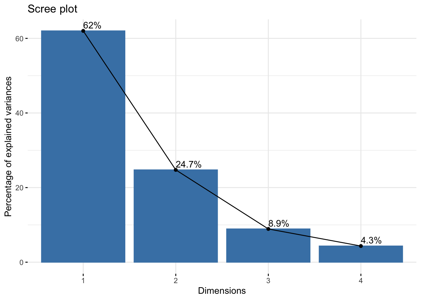
We clearly see here that \(PC1\) encodes 62% of variance, so it does not retain enough information. However, \(PC1\) and \(PC2\) together encode 86.75% of variance in the data, enough to give an informative picture.

The library factoextra has a simple command that can be used to make a nice scree plot:

library(factoextra)
fviz_screeplot(pr.out, addlabels = TRUE)

This is an effective way to visualize the importance of the principal components.

Other useful functions for visualization in the factoextra package are fviz_pca_ind, fviz_pca_var and fviz_pca_biplot.

Task 1b

Explore the functions above (e.g. by typing ?fviz_pca_ind) and describe the kind of plots that you can obtain using them.

Solution to Task 1b

Click for solution

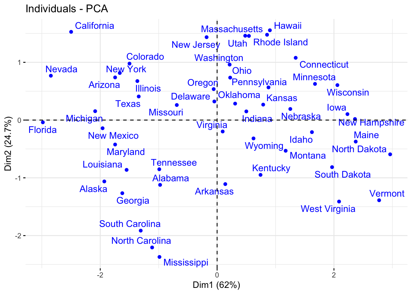
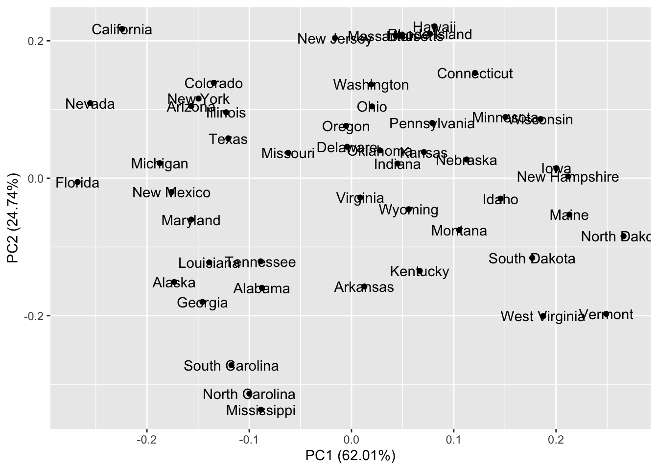
Let us start with fviz_pca_ind(). This command plots the scores of observations of the first two principal components. This is informative, as we saw that \(PC1\) and \(PC2\) explain a big proportion (> 80%) of the variance.

fviz_pca_ind(pr.out, axes = c(1, 2), repel = TRUE,
  col.ind = "blue"
)

We can compare this to the autoplot() function and see that it is just another way of creating the same visualization. The advantage of fviz_pca_ind() is that it is somewhat more flexibile if you want to change options.

#install.packages('ggfortify')
library(ggfortify)

autoplot(pr.out, data = USArrests, label = TRUE) #, label = TRUE

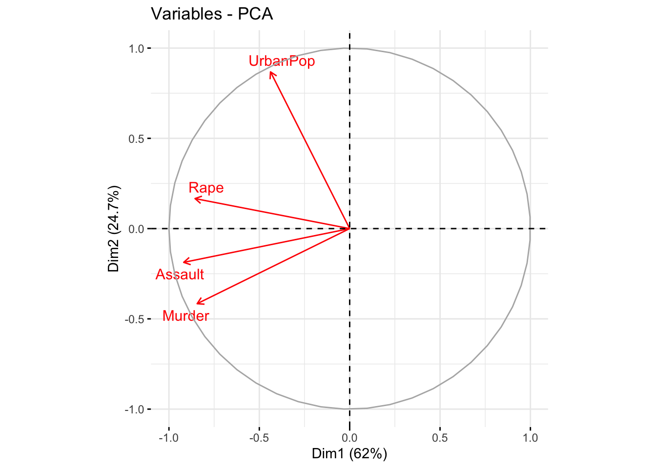
The command fviz_pca_var() plots the loadings of the first two principal components.

fviz_pca_var(pr.out, axes = c(1, 2), repel = TRUE,
  col.var = "red"
)

In the case of USArrests, we can see that the length of the four vectors are very similar. This means that the first two principal components represent quite fairly the original variables. As expected, the crime variables are the one that mostly contribute to the first principal component, while the UrbanPop variable is predominantly contributing to the second principal component.

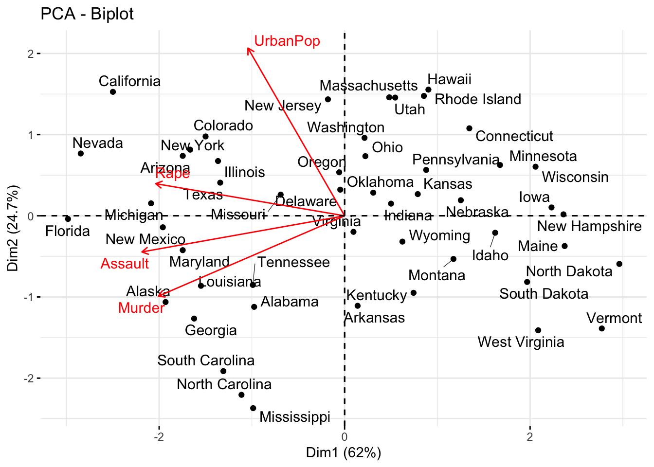
Finally, the fviz_pca_biplot() plots together scores and loading.

fviz_pca_biplot(pr.out, axes = c(1, 2), repel = TRUE,
  col.var = "red"
)

This is very helpful to interpret the data: based only on the plot of the scores, one could think that a higher \(PC1\) score corresponds to higher crime rates. The biplot shows instead that the states on the left of the plot are those with higher crime rates.

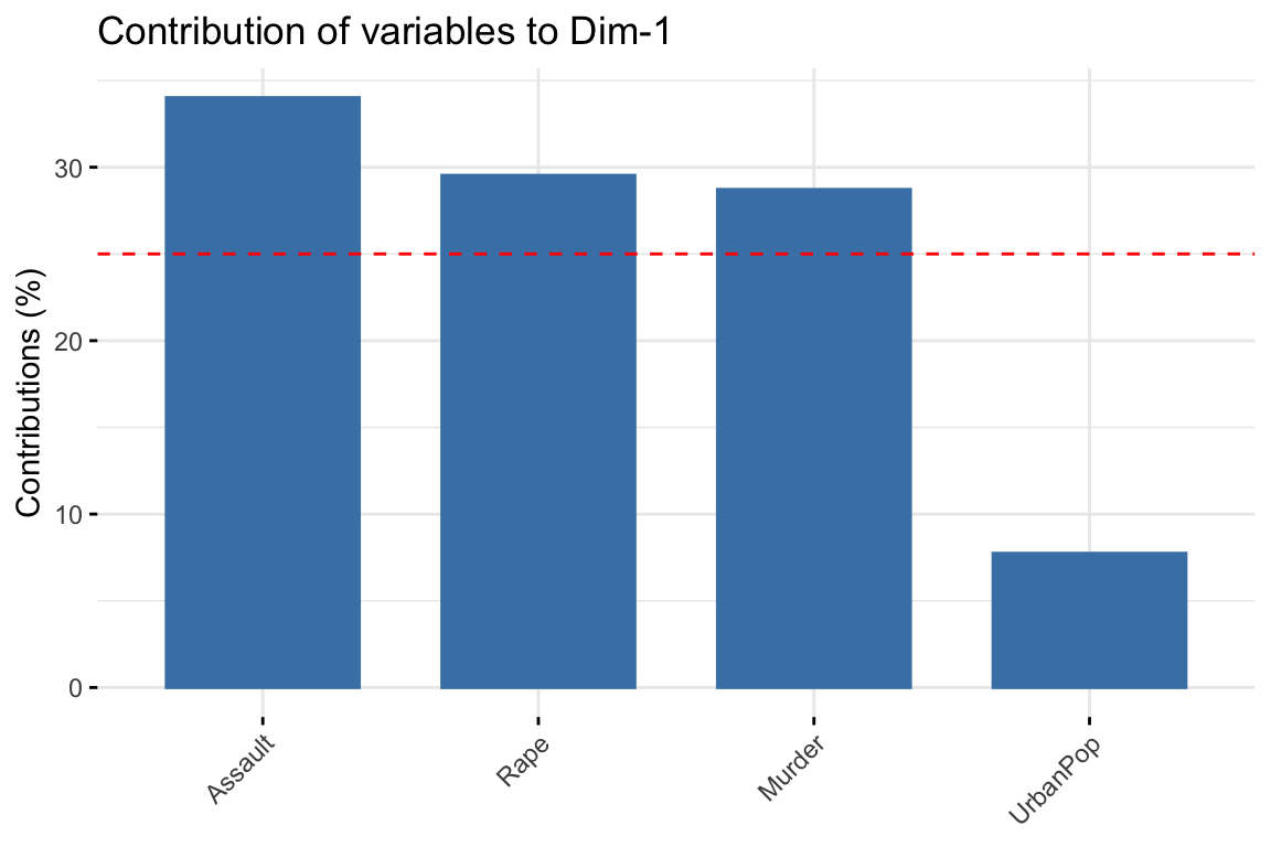
You can plot the contribution of the variables to PC1 as follows:

fviz_contrib(pr.out, choice = "var", axes = 1, top = 10)

Task 1c

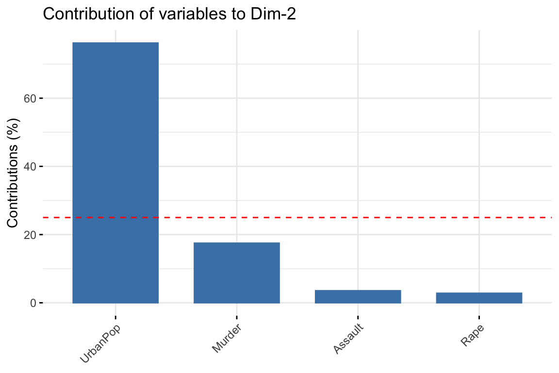
Modify the code to plot the contribution of the variables to PC2.

Solution to Task 1c

Click for solution

# Contributions of variables to PC2
fviz_contrib(pr.out, choice = "var", axes = 2, top = 10)

The library factoextra has commands to quickly extract PCA results for variables. These results include correlation between variables and principal components (cor), quality of representation (cos2), and contributions (contrib). They can be obtained respectively as follows:

var <- get_pca_var(pr.out)
var$cor

              Dim.1      Dim.2      Dim.3       Dim.4
Murder   -0.8439764 -0.4160354  0.2037600  0.27037052
Assault  -0.9184432 -0.1870211  0.1601192 -0.30959159
UrbanPop -0.4381168  0.8683282  0.2257242  0.05575330
Rape     -0.8558394  0.1664602 -0.4883190  0.03707412

var$cos2

             Dim.1     Dim.2      Dim.3       Dim.4
Murder   0.7122962 0.1730854 0.04151814 0.073100217
Assault  0.8435380 0.0349769 0.02563817 0.095846950
UrbanPop 0.1919463 0.7539938 0.05095143 0.003108430
Rape     0.7324611 0.0277090 0.23845544 0.001374491

var$contrib

             Dim.1     Dim.2     Dim.3     Dim.4
Murder   28.718825 17.487524 11.643977 42.149674
Assault  34.010315  3.533859  7.190358 55.265468
UrbanPop  7.739016 76.179065 14.289594  1.792325
Rape     29.531844  2.799553 66.876071  0.792533

If you have a hard time making sense of these numbers, don’t worry: there will be more on this in the lectures.

Exercise 2

Generate n = 200 observations and p=30 variables from a multivariate normal distribution with correlation matrix given as \(corr(x_{i},x_{j}) = \rho^{|i-j|}\). You can create the covariance matrix using

covmat <- function(rho, p) {
  rho^(abs(outer(seq(p), seq(p), "-")))
}

and use the mvrnorm function in MASS package to generate the multivariate Gaussian data.

Task 2a

Take \(\rho=0.95\) and carry out PCA. For reproducibility, set the pseudo-number generator seed = 123. How many PCs are sufficient to retain at least 80% of variance? Comment on your general observation. (Hint: Use the following codes to generate the data called dd.

library(MASS)
set.seed(123)
p = 30
n = 200
cov.e = covmat(0.95, p)
mean.e = rep(0, p)
dd <- mvrnorm(n, mean.e, cov.e)

Solution to Task 2a

Click for solution

prr <- prcomp(dd)
summary(prr)

Importance of components:
                          PC1    PC2    PC3     PC4     PC5     PC6     PC7
Standard deviation     4.1415 2.2933 1.3464 1.00341 0.77935 0.63838 0.48520
Proportion of Variance 0.6179 0.1895 0.0653 0.03627 0.02188 0.01468 0.00848
Cumulative Proportion  0.6179 0.8073 0.8726 0.90886 0.93074 0.94542 0.95390
                           PC8     PC9    PC10    PC11    PC12    PC13   PC14
Standard deviation     0.41615 0.40216 0.37139 0.29564 0.29060 0.26536 0.2469
Proportion of Variance 0.00624 0.00583 0.00497 0.00315 0.00304 0.00254 0.0022
Cumulative Proportion  0.96014 0.96597 0.97093 0.97408 0.97712 0.97966 0.9819
                          PC15    PC16    PC17    PC18    PC19    PC20    PC21
Standard deviation     0.24380 0.22571 0.21583 0.20360 0.18959 0.18087 0.17804
Proportion of Variance 0.00214 0.00184 0.00168 0.00149 0.00129 0.00118 0.00114
Cumulative Proportion  0.98400 0.98583 0.98751 0.98900 0.99030 0.99148 0.99262
                         PC22    PC23    PC24    PC25    PC26    PC27   PC28
Standard deviation     0.1744 0.16711 0.16001 0.15574 0.15240 0.14561 0.1390
Proportion of Variance 0.0011 0.00101 0.00092 0.00087 0.00084 0.00076 0.0007
Cumulative Proportion  0.9937 0.99472 0.99564 0.99652 0.99735 0.99812 0.9988
                          PC29    PC30
Standard deviation     0.12848 0.12825
Proportion of Variance 0.00059 0.00059
Cumulative Proportion  0.99941 1.00000

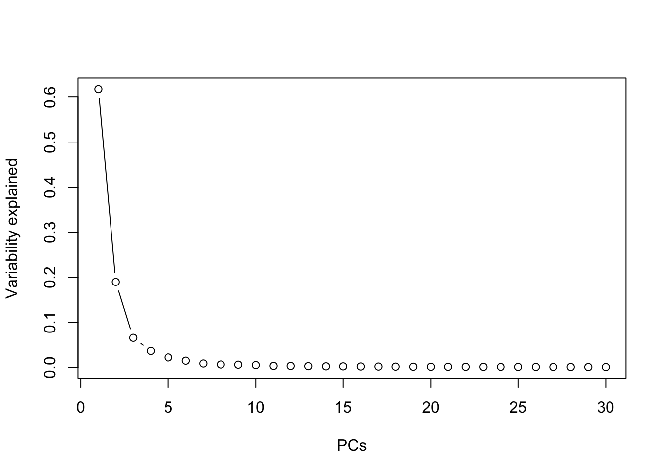
plot(summary(prr)$importance[2,], type="b", xlab="PCs", ylab="Variability explained")

The summary shows that 2 components are enough to keep 80% of the variability in data.

Task 2b

Take \(\rho=0.2\) and carry out PCA. As done before, use the pseudo-number generator, seed = 123 for reproducibility. How many PCs are sufficient to retain at least 80% of variance? Compare your results with the case of \(\rho=0.95\).

Solution to task 2b

Click for solution

library(MASS)
set.seed(123)
p = 30
n = 200
cov.e = covmat(0.2, p)
mean.e = rep(0, p)
dd <- mvrnorm(n, mean.e, cov.e)

prr <- prcomp(dd)
summary(prr)

Importance of components:
                           PC1     PC2     PC3     PC4     PC5     PC6     PC7
Standard deviation     1.46267 1.33775 1.32938 1.28976 1.22917 1.17781 1.17183
Proportion of Variance 0.07223 0.06042 0.05966 0.05616 0.05101 0.04683 0.04636
Cumulative Proportion  0.07223 0.13265 0.19231 0.24847 0.29948 0.34631 0.39267
                           PC8     PC9   PC10    PC11    PC12    PC13    PC14
Standard deviation     1.16283 1.13430 1.1074 1.05365 1.03779 1.01332 0.99861
Proportion of Variance 0.04565 0.04344 0.0414 0.03748 0.03636 0.03467 0.03367
Cumulative Proportion  0.43832 0.48176 0.5232 0.56065 0.59701 0.63167 0.66534
                          PC15    PC16    PC17    PC18    PC19    PC20    PC21
Standard deviation     0.96032 0.92220 0.91021 0.88108 0.85584 0.83619 0.81532
Proportion of Variance 0.03114 0.02871 0.02797 0.02621 0.02473 0.02361 0.02244
Cumulative Proportion  0.69648 0.72519 0.75316 0.77937 0.80410 0.82770 0.85015
                          PC22    PC23    PC24    PC25    PC26    PC27    PC28
Standard deviation     0.78841 0.75942 0.74078 0.71840 0.70589 0.69243 0.66375
Proportion of Variance 0.02099 0.01947 0.01853 0.01742 0.01682 0.01619 0.01487
Cumulative Proportion  0.87113 0.89060 0.90913 0.92655 0.94338 0.95956 0.97444
                          PC29    PC30
Standard deviation     0.62502 0.60544
Proportion of Variance 0.01319 0.01238
Cumulative Proportion  0.98762 1.00000

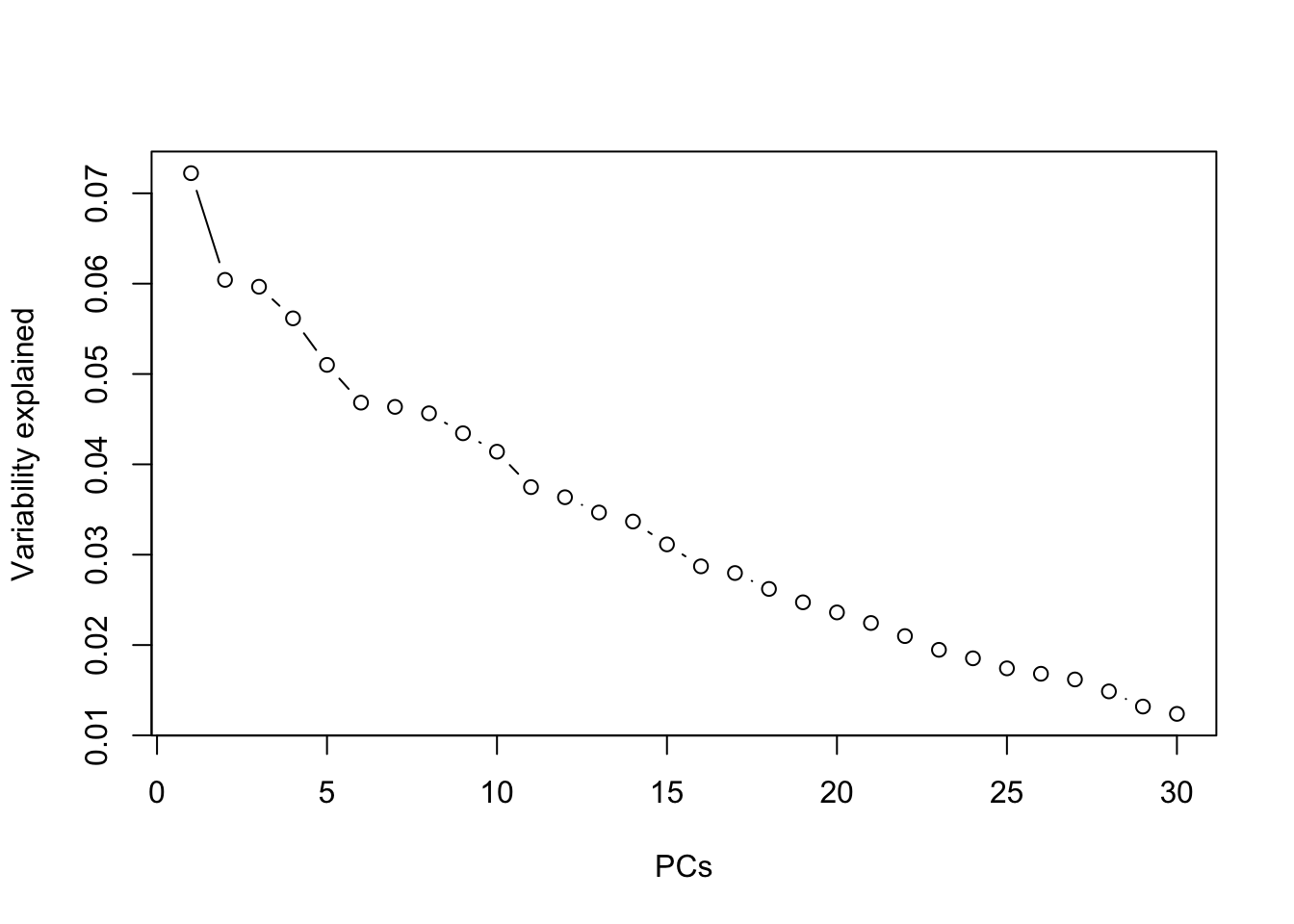
plot(summary(prr)$importance[2,], type="b", xlab="PCs", ylab="Variability explained")

The summary shows that 19 components are needed to keep 80% of the variability in data. This shows that the higher the correlation, the higher the redundancy in the data in which case PCA becomes more useful and gives more clear interpretation.

Exercise 3

One of the many uses of PCA is principal component regression (PCR). We will get a taste of how this works on the Iris data.

We have seen that Sepal length is highly correlated with Petal length and Petal width. Suppose that we want to carryout regression analysis between Sepal length (response variable) and the three remaining variables (covariates). Then we can use PCA to improve our analysis.

Task 3a

Perform the PCA and find the scores of the principal components of the covariates.

Solution to task 3a

Click for solution

iris.pca <- prcomp(iris[,2:4], scale=TRUE)

The rotation matrix is given by

iris.pca$rotation

                    PC1        PC2         PC3
Sepal.Width  -0.4181177 -0.9067335  0.05488053
Petal.Length  0.6482670 -0.2555198  0.71725833
Petal.Width   0.6363391 -0.3354757 -0.69464280

and the scores by

iris.pca$x

              PC1          PC2          PC3
  [1,] -2.1248387 -0.139743260  0.008370721
  [2,] -1.6451988  0.900407772 -0.054584971
  [3,] -1.8737775  0.498821958 -0.070033694
  [4,] -1.7044039  0.677902966 -0.001362832
  [5,] -2.2207666 -0.347773466  0.020961859
  [6,] -2.2314161 -1.103311779 -0.001635822
  [7,] -1.9454276  0.024274998 -0.095352466
  [8,] -1.9921879  0.053812348  0.036410583
  [9,] -1.5492708  1.108437978 -0.067176109
 [10,] -1.7878870  0.721914915  0.089769216
 [11,] -2.2799718 -0.570278271  0.074183997
 [12,] -1.9554651  0.039337749  0.077041583
 [13,] -1.7286818  0.944419721  0.036547077
 [14,] -1.8388502  0.987843518 -0.085345923
 [15,] -2.6779242 -1.150945093 -0.009935588
 [16,] -2.7845016 -2.114513613 -0.019942131
 [17,] -2.3783073 -1.045413383 -0.164159822
 [18,] -2.0413556 -0.183755209 -0.082761327
 [19,] -2.2189712 -0.851269624  0.076905088
 [20,] -2.2924168 -0.822320426 -0.004356912
 [21,] -1.9187423  0.024863150  0.117672583
 [22,] -2.1130058 -0.658302169 -0.108080099
 [23,] -2.3676579 -0.289875070 -0.141562142
 [24,] -1.5723652  0.100857509 -0.168314699
 [25,] -1.8452967 -0.004086048  0.198934583
 [26,] -1.5717531  0.871458574  0.026677030
 [27,] -1.7884990 -0.048686149 -0.105222513
 [28,] -2.0881159 -0.154217859  0.049001721
 [29,] -2.0289107  0.068286947 -0.004220418
 [30,] -1.7636091  0.455398161  0.051859306
 [31,] -1.6676811  0.663428368  0.039268168
 [32,] -1.8252218 -0.034211550 -0.145853513
 [33,] -2.7471668 -1.358387147  0.215680599
 [34,] -2.7963345 -1.595954703  0.096508689
 [35,] -1.7044039  0.677902966 -0.001362832
 [36,] -1.9105003  0.513296557 -0.110664695
 [37,] -2.1615615 -0.125268661 -0.032260280
 [38,] -2.3042497 -0.303761517  0.112093907
 [39,] -1.6819216  0.914882371 -0.095215971
 [40,] -1.9921879  0.053812348  0.036410583
 [41,] -2.0780784 -0.169280610 -0.123392328
 [42,] -0.9269427  2.327081865 -0.274485987
 [43,] -1.8737775  0.498821958 -0.070033694
 [44,] -1.7174609 -0.344740253 -0.274895471
 [45,] -2.0620425 -0.924230771  0.067035040
 [46,] -1.5617157  0.856395823 -0.145717019
 [47,] -2.3391770 -0.792783076  0.127406136
 [48,] -1.8370547  0.484347359 -0.029402694
 [49,] -2.2799718 -0.570278271  0.074183997
 [50,] -1.9329827  0.276317153 -0.016811556
 [51,]  0.3765942 -0.521457794  0.217835736
 [52,]  0.3866316 -0.536520545  0.045441688
 [53,]  0.6294508 -0.386388735  0.195374550
 [54,]  0.8994033  1.496148204 -0.088769462
 [55,]  0.8070663  0.281125681  0.035708135
 [56,]  0.6033775  0.383624178  0.177341231
 [57,]  0.4476323 -0.817511898  0.048162778
 [58,]  0.2959666  1.521476037 -0.087199181
 [59,]  0.5441723  0.161119373  0.230563369
 [60,]  0.5624516  0.634490029 -0.170167957
 [61,]  0.7531242  2.324647664 -0.056301734
 [62,]  0.4683191 -0.077036336 -0.101633589
 [63,]  0.7448822  1.836214257  0.172035544
 [64,]  0.6643781  0.102632825  0.180062321
 [65,]  0.1769442  0.305865362 -0.175746633
 [66,]  0.3623537 -0.270003791  0.083351597
 [67,]  0.5784876 -0.120460133  0.020259411
 [68,]  0.3019651  0.781588627  0.275622236
 [69,]  1.3459114  1.543781517 -0.080469695
 [70,]  0.5038585  1.182586288  0.078045911
 [71,]  0.7472491 -0.711980189 -0.106061456
 [72,]  0.4197634  0.455997173 -0.025813770
 [73,]  1.2050187  0.861792503  0.119827721
 [74,]  0.5933400  0.398686929  0.349735279
 [75,]  0.4340039  0.204543170  0.108670369
 [76,]  0.4582817 -0.061973585  0.070760459
 [77,]  0.7970289  0.296188432  0.208102183
 [78,]  0.9290676 -0.280857025  0.041150316
 [79,]  0.6744155  0.087570074  0.007668273
 [80,]  0.1775563  1.076466427  0.019245096
 [81,]  0.5630637  1.405091093  0.024823772
 [82,]  0.4428579  1.463577641  0.075324820
 [83,]  0.3954856  0.722513927  0.012096139
 [84,]  1.1700913  0.372770943  0.135139949
 [85,]  0.5784876 -0.120460133  0.020259411
 [86,]  0.2782587 -0.996592907 -0.020508084
 [87,]  0.5560052 -0.357439537  0.114112550
 [88,]  1.0462946  1.438249808  0.073754539
 [89,]  0.2646303  0.025462161  0.039999506
 [90,]  0.7075474  1.080087791 -0.063587185
 [91,]  0.6750276  0.858171138  0.202660002
 [92,]  0.5317273 -0.090922783  0.152022459
 [93,]  0.5281364  0.916069534  0.040136001
 [94,]  0.3918946  1.729506244 -0.099790319
 [95,]  0.5891370  0.635078181  0.042857092
 [96,]  0.2178701  0.054999511  0.171762555
 [97,]  0.3972811  0.219017768  0.068039368
 [98,]  0.4340039  0.204543170  0.108670369
 [99,]  0.1733533  1.312857679 -0.287633091
[100,]  0.4564862  0.441522574  0.014817230
[101,]  1.6763760 -1.401789225 -0.243822651
[102,]  1.4205404  0.240735097 -0.138256195
[103,]  1.5935050 -0.587176212  0.042301126
[104,]  1.3288155 -0.203686362  0.181213131
[105,]  1.6402652 -0.616713562 -0.089461922
[106,]  1.8505646 -0.688498405  0.326718127
[107,]  1.2250935  0.831667001 -0.224960376
[108,]  1.5858751 -0.305008555  0.465630132
[109,]  1.7859730  0.599485265  0.212110578
[110,]  1.4253148 -2.040354443 -0.165418236
[111,]  1.0243836 -0.843427884 -0.166432551
[112,]  1.4939861  0.211785899 -0.056994194
[113,]  1.4466138 -0.529277816 -0.120222875
[114,]  1.6591566  0.627258159 -0.295201519
[115,]  1.7420276 -0.187354854 -0.581325296
[116,]  1.3482783 -1.004412928 -0.358566695
[117,]  1.1961647 -0.397241969  0.153173269
[118,]  1.2033466 -2.411226602  0.376946186
[119,]  2.5114110  0.012174726  0.215982479
[120,]  1.5295254  1.471408523  0.122685306
[121,]  1.4951695 -1.062311324 -0.196042694
[122,]  1.3346499  0.017642139 -0.298059105
[123,]  1.9956603 -0.242900642  0.433298899
[124,]  1.2636118  0.313696243 -0.128386147
[125,]  1.2322754 -1.182317633 -0.001187460
[126,]  1.1879227 -0.885675376  0.381510547
[127,]  1.1309610  0.120140636 -0.156426009
[128,]  0.9758279 -0.310394375 -0.090612732
[129,]  1.6751925 -0.127692002 -0.104774151
[130,]  1.1393670 -0.352641868  0.457330366
[131,]  1.6918405 -0.112041099  0.280644946
[132,]  0.9262121 -2.279778908  0.437317281
[133,]  1.7586756 -0.171703951 -0.195906199
[134,]  0.9906803  0.208752686  0.238863136
[135,]  1.2826673  0.596452053  0.507967908
[136,]  1.8339167 -0.704149308 -0.058700970
[137,]  1.3500738 -1.507909087 -0.302623466
[138,]  1.1002367 -0.605272175  0.165764407
[139,]  0.9391051 -0.295919776 -0.131243732
[140,]  1.3139630 -0.722833423 -0.148262737
[141,]  1.6378577 -0.883818468 -0.340396881
[142,]  1.3707607 -0.767433524 -0.452419834
[143,]  1.4205404  0.240735097 -0.138256195
[144,]  1.5686151 -1.091260522 -0.114780694
[145,]  1.5662076 -1.358365428 -0.365715652
[146,]  1.5034114 -0.573877917 -0.424379972
[147,]  1.5756736  0.671270108 -0.204069471
[148,]  1.2529623 -0.441842070 -0.150983828
[149,]  1.1931451 -1.434947940 -0.292753418
[150,]  1.0492735 -0.339343573 -0.009350732

Task 3b

Run a linear regression by using the lm() command. This carries out the principal component regression (PCR, not PCA!). Use just the first 2 principal components as covariates in the linear regression model. As hinted before, the response variable should be Sepal length.

Solution to task 3b

Click for solution

Z = iris.pca$x[,1:2] # select the first two PCs
iris.lm <- lm(iris$Sepal.Length~Z)
iris.lm

Call:
lm(formula = iris$Sepal.Length ~ Z)

Coefficients:
(Intercept)         ZPC1         ZPC2  
     5.8433       0.4230      -0.4348  

Now, you can transform this coefficient vector to the scale of the original variables as follows (might look mysterious for now: come back and see this again after the lecture!). This gives the final PCR estimator, whose dimension is equal to the total number of original covariates.

iris.pca$rotation[,1:2]%*%matrix(coef(iris.lm)[-1], ncol=1)

                  [,1]
Sepal.Width  0.2173767
Petal.Length 0.3853085
Petal.Width  0.4150270

Task 3c

In practice, we do not need to do PCR ourselves in this way, as this is implemented in the pls R package. Carryout PCR using the pcr function in R (check HERE) and compare the results.

Solution to task 3c

Click for solution

library(pls)
iris.pcr <- pcr(Sepal.Length~ Sepal.Width+Petal.Length+Petal.Width, 2, 
                scale=TRUE, data=iris) # 2 stands for number of principal components used in pcr,
coef(iris.pcr)

, , 2 comps

             Sepal.Length
Sepal.Width     0.2173767
Petal.Length    0.3853085
Petal.Width     0.4150270