Lecture7b: Hierarchical clustering

A small sample of generated data

Let us generate 8 data points in the plane to see how hierarchical clustering is performed on them:

X <- c(-2,-4,-6,0,3,6,7,8)
Y <- c(0,0,2,3,5,6,5,9)
otto.dat <- data.frame(X,Y)

Remember that the input is going to be given by the dissimilarity matrix, not the data set.

diss <- as.matrix(dist(otto.dat))

The smallest distance is between point 6 and point 7 then the algorithm clusters them together. We are now ready to make up an updated data matrix. The entries will now be the clusters, and the distance will be the linkage between them. To illustrate this, let us choose complete linkage. This amounts to replacing rows and columns \(6\) and \(7\) with a single one, representing the maximum of the entries.

diss[6,] <- pmax(diss[6,], diss[7,])
diss[,6] <- pmax(diss[6,], diss[7,])
diss[6,6] <- 0
diss2 <- diss[-7,-7]

We then agglomerate together clusters 1 and 2. Since we need to repeat the same procedure as above, it seems wise to create a specific function that does the job for us.

agglomerate <- function(M,a,b){
  M[a,] <- pmax(M[a,], M[b,])
M[,a] <- pmax(M[a,], M[b,])
M[a,a] <- 0
return(M[-b,-b])
}

Let us check if this works:

diss2 <- agglomerate(diss,6,7)
diss3 <- agglomerate(diss2, 1, 2)

It is now the turn of agglomerating clusters {4} and {5} (which are now the third and fourth rows/columns in the matrix!)

diss4 <- agglomerate(diss3, 3, 4)

Then is the turn of {6,7} and {8}

diss5 <- agglomerate(diss4, 4, 5)

Then is the turn of {1,2} and {3}

diss6 <- agglomerate(diss5, 1, 2)

Then is the turn of {1,2,3} and {4,5}

diss7 <- agglomerate(diss6, 1, 2)

Finally, we create a unique cluster containing everything:

diss8 <- agglomerate(diss7, 1, 2)

Let’s now check that our algorithm coincides with the one implemented in R:

hc <- hclust(dist(otto.dat), method = "complete")
plot(hc, bty="7")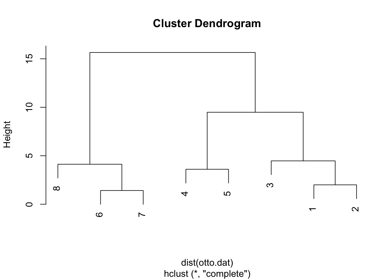

USArrests data

Let us now get a taste of how hierarchical clustering works on real worlds data sets. For our convenience, we’ll try it on a bulit-in data set, the USArrests one.

data("USArrests")
# Compute distances and hierarchical clustering
dd <- dist(scale(USArrests), method = "euclidean")
hc <- hclust(dd, method = "complete")

hcut <- cutree(hc, k = 4)
head(hcut)

   Alabama     Alaska    Arizona   Arkansas California   Colorado 
         1          1          2          3          2          2 

table(hcut)# Number of members in each cluster

hcut
 1  2  3  4 
 8 11 21 10 

# Get the names for the members of cluster 1
rownames(USArrests)[hcut == 1]

[1] "Alabama"        "Alaska"         "Georgia"        "Louisiana"     
[5] "Mississippi"    "North Carolina" "South Carolina" "Tennessee"     

As for visualization, we have different options.

We can plot the output as a dendrogram

plot(hc, hang = -1, cex = 0.6)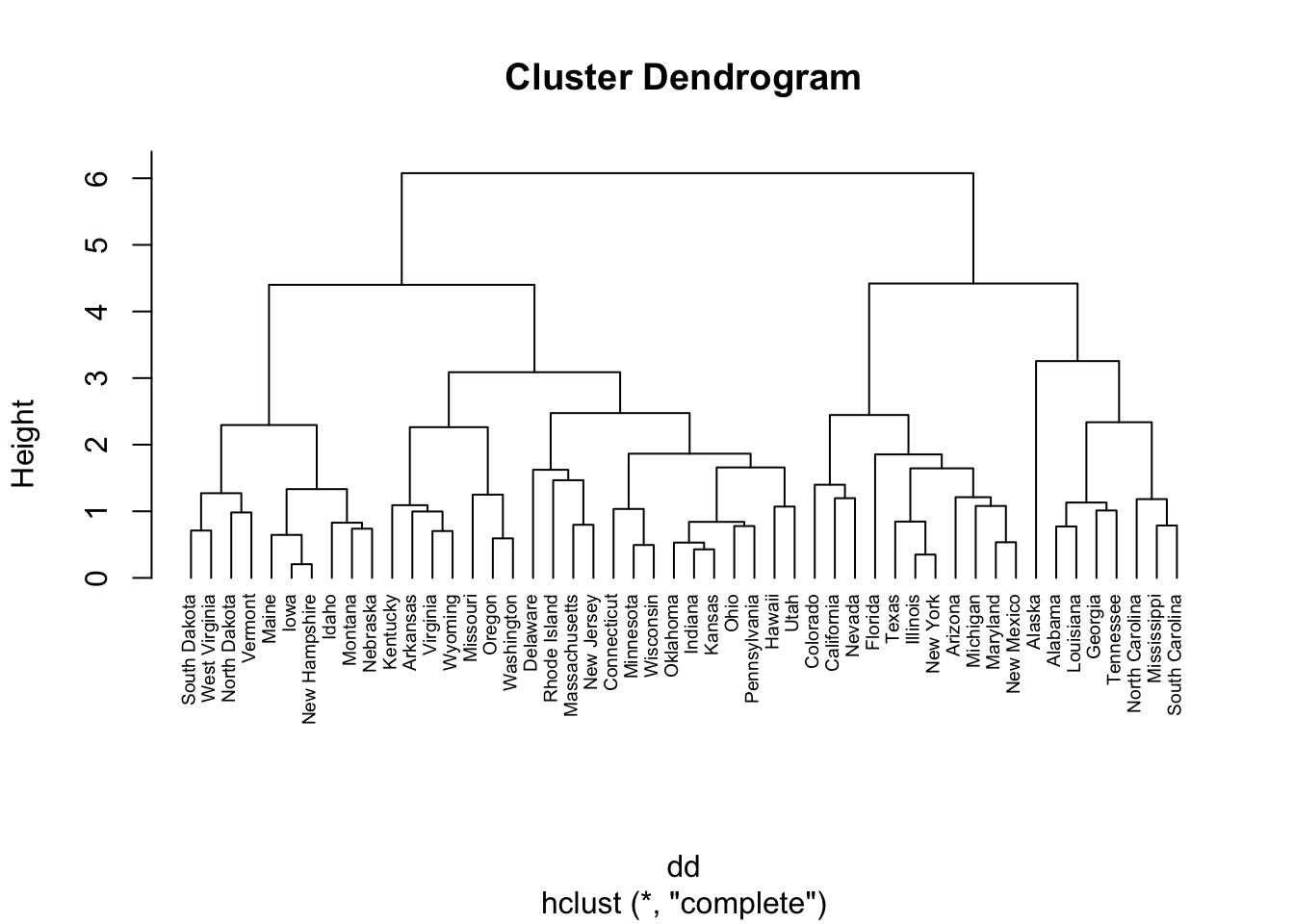

We can plot the output as a circular dendrogram

library('ape')
colors = c("red", "blue", "green", "black")
clus4 = cutree(hc, 4)
plot(as.phylo(hc), type = "fan", tip.color = colors[clus4],label.offset = 0.1, cex = 0.7)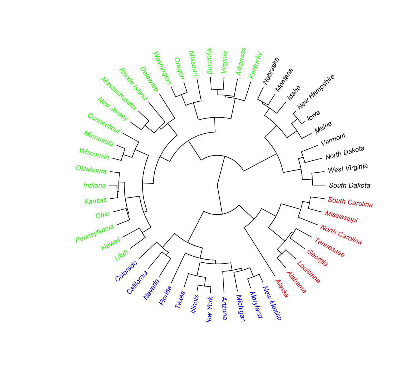

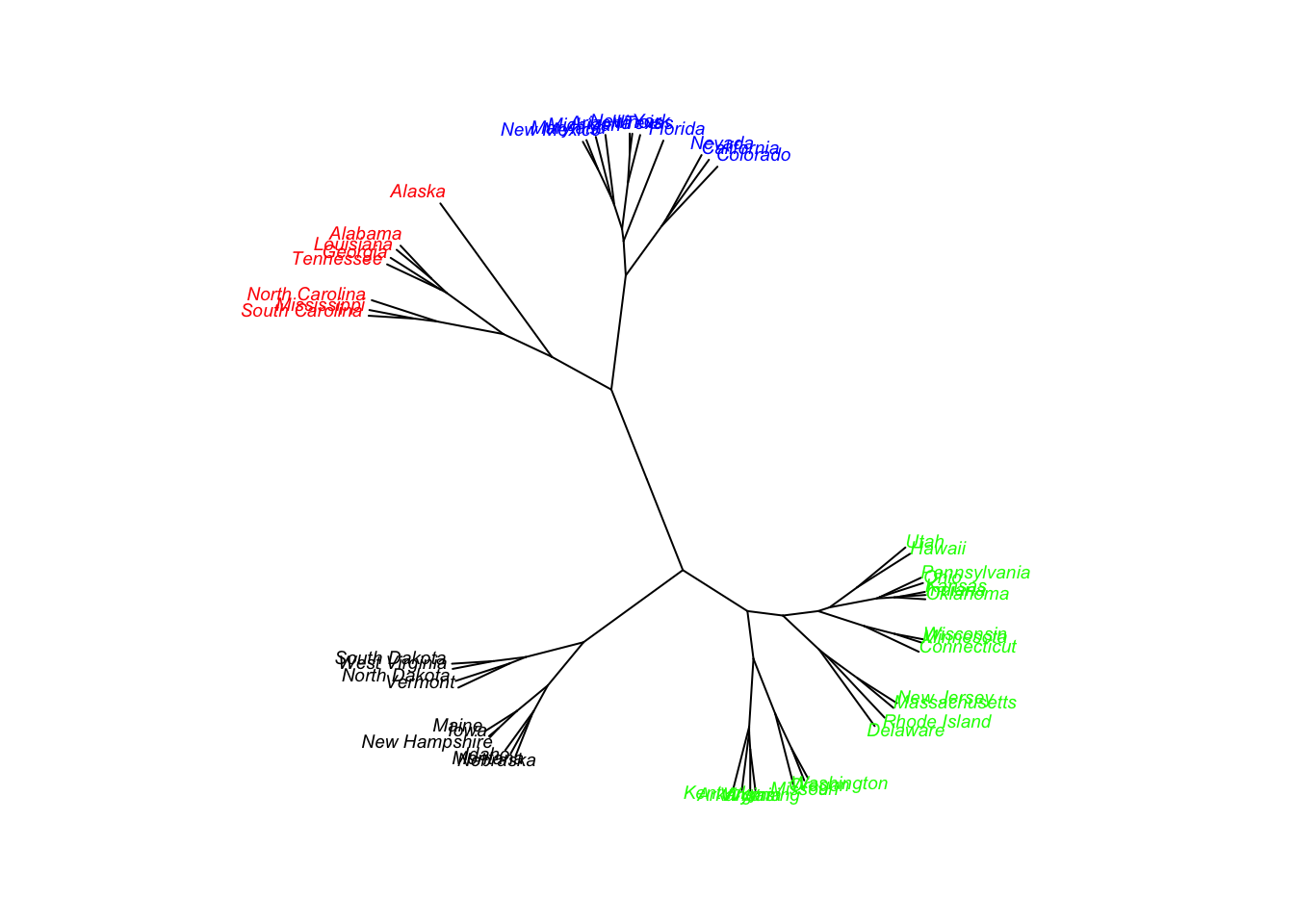
We can plot the output as an unrooted binary tree

plot(as.phylo(hc), type = "unrooted", tip.color = colors[clus4], cex = 0.6,
     no.margin = TRUE)